31 known samples across three batches and 9 test samples. BSE, Inlens and ETD/SE measurements, methods and comparisons.
Abstract
We assess electrode-batch similarity using 13 physical descriptors and a porosity uncertainty estimate from 31 labelled crops and 9 test samples. Joint segmentation of BSE, Inlens and ETD/SE images measures phase area fractions, pore structure, and silicon-region geometry and spatial variation. Test vectors are assigned to the nearest standardised batch mean. Leave-one-crop-out validation correctly assigns 18 of 31 crops (58.1%). Confidence bands report validation precision for each predicted batch. The report provides individual measurements, segmentation figures and reproducible calculations. Segmentation boundaries and crop independence remain unvalidated; manufacturing acceptance criteria have not been established.
1. Introduction
Batch 3 represents the material promised by the supplier. Batches 1 and 2 contain subsequent, deliberately assembled patterns of variation; neither is labelled better or worse. The challenge evaluates whether each held-out image can be assigned to Batch 1, 2 or 3 with confidence and a physical explanation. Distinguishing Batch 1 from Batch 2 matters as much as distinguishing either from the reference.
We compare four feature families: phase area fractions, pore geometry, silicon-region size and shape, and silicon spatial variation. The organisers describe the data as crops from approximately 15 original electrode images, arranged into artificial batches. This is a test of recognising microstructural patterns. Establishing manufacturing acceptance limits or performance on genuinely new material populations would require separate validation.
These measurements describe how much of each assigned phase is present, the dimensions and directionality of pore space, and the geometry and distribution of silicon-labelled regions. Each value can be traced to a mask or geometric calculation. Their physical interpretation is limited by the two-dimensional images and the phase assignments; they do not directly measure transport or establish a manufacturing defect.
Each sample is one image crop observed with three detectors, not three independent observations. The same extraction is applied to known and test samples, and each assignment is accompanied by its measured physical features.
2. Physical interpretation and glossary
What the electrode characteristics mean, why we measured them, and how each measurement was obtained.
Overall rationale
A single number such as porosity cannot fully describe an electrode, because microstructure can change in ways one measure misses. The current report covers phase composition, pore organisation, silicon particle size and shape, and silicon particle spatial variation. These complementary families target different aspects of the microstructure (our interpretation).
2D estimates of 3D properties can be biased and orientation-dependent. Tortuosity and 3D connectivity cannot be recovered reliably from these sections. Compare batches in the same orientation (our interpretation). Taiwo et al.
Representativity is property-specific: an image representative for phase fraction need not be representative for interface. Dahari et al.
Uncertainty estimates assume perfect segmentation; segmentation error can exceed finite-image sampling error. Dahari et al.
(a) Phase area fractions
A phase is a distinct material or pore region, such as graphite or void space. Its area fraction is the percentage of the image assigned to it.
Pore, graphite and silicon-labelled area fractions, with a separate carbon-binder allocation.
Physical meaning
An electrode contains solid material and void space. In a conventional liquid-electrolyte cell, electrolyte in the pores carries ions; active material stores lithium; conductive carbon provides electronic connections. Area fractions describe how much of each assigned region is visible in a cross-section. The project lead identifies the silicon particles as silicon active material; their area fraction is not silicon weight fraction.
Phase
A distinguishable constituent or region. Phase names use the supplied material identity; the intensity-derived mask boundaries remain unvalidated.
Area fraction
The share of the analysed two-dimensional image assigned to a region. It is not a mass fraction or a directly measured three-dimensional volume fraction.
Porosity
The area fraction assigned to pore space in this report.
Carbon-binder domain (CBD)
Conductive carbon and polymer binder associated with particle contacts. Our CBD value is an intensity-based allocation within the pore-labelled cluster.
Relevance to electrode performance
The balance of active material, pore space and conductive material affects how much charge an electrode can store and how ions and electrons reach reaction sites. In a liquid-electrolyte electrode, pore space accommodates the ionic conductor, while solid active material supplies storage sites. More porosity is therefore not automatically better: transport and active-material loading must both be considered.
Literature basis
Silicon expansion and electrochemical–mechanical interactions affect degradation in silicon–graphite composites, motivating separate tracking of silicon content. Moon et al. (2021).
In reconstructed LiCoO₂ cathodes, pore space, active material and carbon-binder regions serve distinct ionic transport, lithium-storage and electronic transport roles. Including carbon-binder nanoporosity changed the calculated ionic conduction. Zielke et al. (2015).
Experiments with graphite particle-size mixtures linked changes in packing and porosity with changes in electrochemical behaviour. Choi et al. (2023).
Scope for this analysis: These studies motivate measuring phase proportions. They do not validate our image-intensity labels, CBD allocation or a batch acceptance threshold.
How we defined and measured each phase
Retain the central 80% of image rows and smooth each detector with Gaussian σ = 1 pixel. Standardize BSE, Inlens and ETD/SE separately within each crop, then cluster their joint pixel vectors with three-class KMeans. Order the fitted centroids by their BSE coordinate to label pore, graphite and silicon.
Current three-channel phase assignment. Each pixel is assigned to its nearest fitted centroid in standardized BSE/Inlens/ETD or SE intensity space.
Reported region
Pixel assignment
Pore-labelled area
Joint cluster whose fitted centroid has the lowest BSE coordinate.
Graphite-labelled matrix
Joint cluster whose fitted centroid has the intermediate BSE coordinate.
Silicon particles
Joint cluster whose fitted centroid has the highest BSE coordinate. Silicon identity is supplied by the project lead; mask boundaries remain provisional.
Carbon-binder allocation
Within the pore-labelled cluster, smoothed Inlens intensity above its within-cluster median. Pixels at or below that median form the open-pore subset.
For every reported region, divide its pixel count by the full cropped image area and multiply by 100. Porosity uses the entire pore mask from the selected segmentation, including its CBD allocation. The Inlens median split is used within the pore-labelled cluster. Combined segmentation and its assumptions.
fk=100NcropNk[%]
Pore, graphite and silicon-labelled fractions sum to 100%. CBD is a subset of the pore-labelled area, so adding it again would double count. The median split has not been independently calibrated as a binder measurement.
The scale and directional organisation of the empty regions visible between solid material.
Correlation length scale, horizontal and vertical pore chords, and chord anisotropy.
Physical meaning
The pore network provides space for electrolyte. Its geometry affects how ions can move through an electrode. We describe the patterns visible in a cross-section, including whether pore runs are longer horizontally or vertically.
Chord length
The length of an uninterrupted straight segment through a pore in the image. It describes a line through the void, not a pore diameter or a three-dimensional throat.
Anisotropy
A difference with direction. Here it is the ratio of mean horizontal to mean vertical pore chord length.
Correlation length
A spatial scale derived from how pore labels co-vary at separated positions. It is distinct from the mean chord length.
Tortuosity
The transport penalty associated with the geometry of connected paths. It is not measured by this two-dimensional analysis.
Relevance to electrode performance
Ion transport depends on how pore space is arranged and connected, not only on its amount. Direction-dependent pathways can produce different transport resistance through the electrode thickness and along its plane, affecting rate capability. Our chords describe visible directional geometry; they do not measure transport resistance or tortuosity. The correlation scale characterises spatial organisation and representativity, rather than providing a direct performance score.
Literature basis
An analytical composite-electrode model identifies initial porosity and expansion tolerance as design factors. It does not validate our pore chords as a measure of silicon expansion. Otero et al. (2018).
Tomography and diffusion simulations linked particle shape and alignment to direction-dependent tortuosity, showing why transport cannot be described by porosity alone. Ebner et al. (2014).
Graphite-anode tomography found different tortuosity and surface area in aged and pristine material despite similar porosity. Mitsch et al. (2014).
The two-point correlation function was used to estimate phase-fraction representativity. This supports our correlation length and porosity interval, rather than a direct performance prediction. Dahari et al. (2025).
Scope for this analysis: The transport studies motivate measuring pore geometry. They do not establish that our two-dimensional chord lengths or chord ratio measure tortuosity or predict rate capability.
How we calculated it
On the full pore-labelled cluster, including its CBD allocation, measure uninterrupted runs along every 40th row and column. Multiply pixel lengths by 0.025 µm/pixel and take the mean in each direction. Divide the horizontal mean by the vertical mean. ImageRep separately calculates the correlation length scale from the same mask.
Lx=sℓx,Ly=sℓy,R=Lx/Ly
A longer chord does not establish better transport. These measurements do not recover three-dimensional connectivity or tortuosity. Interpreting image x and y as electrode directions requires known specimen orientation.
The dimensions and elongation of connected silicon particle regions in the image.
Silicon-labelled component aspect ratio and equivalent-diameter percentiles D10, D50 and D90.
Physical meaning
A silicon particle region is a connected component of the silicon-labelled cluster. Size and shape measurements describe this population so that batches can be compared even when their total silicon area is similar. Silicon identity follows the project lead’s identification; the cluster boundaries remain provisional.
Equivalent diameter
The diameter of a circle with the same area as a segmented region.
D10, D50 and D90
The diameters below which 10%, 50% and 90% of the measured objects fall. Every retained object contributes one observation.
Aspect ratio
The major-axis length divided by the minor-axis length of an ellipse fitted to an object's shape. Larger values indicate more elongated regions.
Relevance to electrode performance
The size and shape of identified electrode particles can affect packing and pore geometry, with consequences for transport. Silicon particle size has been linked to degradation in silicon–graphite anodes. Our size and shape measurements describe the segmented regions, not their cycling performance.
Literature basis
Silicon particle size and graphite hardness affected degradation in silicon–graphite anodes; this supports distinguishing silicon-region size from graphite-particle size. Moon et al. (2021).
Changing the size distribution of identified graphite particles altered packing, porosity and electrochemical behaviour in fabricated anodes. Choi et al. (2023).
Particle shape and fabrication-induced alignment were linked to directional tortuosity using tomography and diffusion simulations. Ebner et al. (2014).
Scope for this analysis: Silicon size may be relevant to degradation, but our 2D regions may contain merged particles. Silicon aspect ratio remains exploratory; no performance or damage threshold is established.
How we calculated it
Label connected components in the silicon mask and retain components of at least 10 pixels. Convert their areas to equivalent-circle diameters and calculate unweighted diameter percentiles. Average major-axis/minor-axis ratios, with a one-pixel minimum denominator and zero minor axes excluded.
deq=sπ4A,Ar=mean(max(b,1)a)
A is component area in pixels; a and b are ellipse axes in pixels. These objects are not separated by watershed, so touching regions may form one component. No defect threshold is inferred from their geometry.
How unevenly silicon particles are distributed across different parts of an image.
Standard deviation of local silicon particle area fractions across 16 image regions.
Physical meaning
Two cross-sections can contain the same overall silicon particle fraction but distribute it differently: one relatively evenly, the other in concentrated regions. A spatial measurement captures this difference in local silicon coverage. It does not measure binder distribution or identify why clustering occurred.
Local area fraction
The percentage of one image region occupied by the silicon particle mask.
Spatial variation
Differences in local area fraction between regions. This describes uneven coverage, rather than uncertainty in the overall mean.
Percentage points
The units of differences between percentages. Variation from 5% to 8% is a difference of 3 percentage points.
Relevance to electrode performance
Spatially uneven electrode microstructure can create local differences in transport and reaction conditions, so equal average composition does not guarantee equal electrochemical behaviour. Our statistic asks whether silicon coverage is uniform across an image. It is a screening measurement of heterogeneity, not a validated predictor of current distribution, capacity or a mixing defect.
Literature basis
Wet ball milling conditions affected silicon agglomeration and distribution. This motivates examining silicon coverage, but does not validate our 4 × 4 statistic as a processing diagnosis. Cabello et al. (2020).
Tomography and electrochemical simulations of commercial graphite anodes showed uneven current distributions and higher local overpotentials in heterogeneous structures compared with a more uniform comparison. Müller et al. (2018).
Scope for this analysis: This supports examining spatial heterogeneity. It does not validate our 4 × 4 silicon-particle statistic as a predictor of current distribution, capacity, mixing defects or failure.
How we calculated it
Divide the silicon particle mask into 4 × 4 tiles. Compute the silicon particle area percentage in each tile, then take the population standard deviation of the 16 percentages (ddof = 0).
σinc=161j=1∑16(fj−f)2
This value depends on the tile size, image crop and segmentation. Higher variation indicates less uniform local coverage at that scale; it does not identify the manufacturing cause.
These four families contain 13 physical descriptors. Porosity uncertainty is reported alongside them as information about measurement precision. Taiwo et al. (2016) explain why two-dimensional sections cannot resolve all three-dimensional geometry and connectivity.
3. Methods
The pipeline jointly segments BSE, Inlens and ETD/SE, then extracts one 13-dimensional physical descriptor vector per sample. Porosity uncertainty is reported separately. Calculation links open the extraction code below.
From image to vector
Three-channel KMeans assigns each pixel to a pore, graphite or silicon-labelled region. Physical measurements are calculated from these masks.
1. Prepare
Match BSE, Inlens and ETD/SE by sample. Retain the first stored intensity channel, crop the central 80% of rows and smooth each detector with Gaussian σ = 1 pixel. Use 0.025 µm/pixel.
2. Segment
Standardize each detector within the crop. Fit three-class KMeans to sampled joint pixel vectors, initialized from BSE Multi-Otsu. Order fitted centroids by their BSE coordinate, then assign every cropped pixel.
3. Measure
Count phase pixels and retain the Inlens median CBD allocation. Apply ImageRep and chord measurements to the full pore mask; measure silicon components and variation across 16 tiles.
4. Export
Save 13 physical descriptors and porosity uncertainty for each sample and segmentation. Retain full precision for comparisons; round only for display.
Image preparation and three-detector segmentation
Inputs and image preparation
Detector images and crop
Match BSE, Inlens and ETD images by sample identifier. Four known samples use the filename label SE for the third detector; this naming convention does not establish identical acquisition settings. Require equal pixel grids and inspect detector correspondence before stacking. No automatic registration or resampling is applied.
Select the first stored intensity channel, retain rows int(0.1*h):int(0.9*h) and every column, then smooth each detector with Gaussian sigma=1.0, preserve_range=True. The pixel-size setting is 0.025 µm/pixel; it has not been independently verified from the TIFF metadata. Image preparation code.
Joint segmentation
Standardize each smoothed detector within its full crop by subtracting its mean and dividing by its population standard deviation (ddof=0). Each pixel becomes a three-component vector of standardized BSE, Inlens and ETD/SE intensities.
Select up to 100,000 pixel coordinates without replacement using NumPy seed 42. Three-class Multi-Otsu on the smoothed BSE image provides initial labels. Initialize each joint centroid as the mean sampled vector in its BSE class.
Fit three-cluster K-means using those centroids, n_init=1, random_state=42, max_iter=300, tol=1e-4 and the Lloyd algorithm. Assign every cropped pixel to its nearest fitted centroid.
Order the fitted centroids by their BSE coordinate. Label the clusters pore, graphite matrix and silicon from lowest to highest BSE centroid intensity.
Centroids and channel normalization are fitted separately to each image. The algorithm, initialization rule and settings stay fixed for known and test images. Constant or nonfinite channels, missing initialization classes, collapsed clusters or reaching the iteration limit stop extraction. Segmentation code.
Phase definitions and carbon-binder allocation
The three clusters are mutually exclusive image-based phase assignments. The project lead identifies the bright material as silicon; the intensity rule does not validate every segmented boundary. Every phase fraction uses the full cropped image as its denominator.
Within the pore-labelled mask, calculate the median smoothed Inlens intensity. Pixels above this median form the carbon-binder allocation (CBD); pixels at or below it form the open-pore subset. CBD is approximately half the pore area by construction and is not an independently calibrated binder measurement.
The masks satisfy pore = open_pore + CBD and pore + graphite + silicon = 100%. CBD must not be added again as a fourth independent composition fraction. All pore geometry and ImageRep calculations use the entire pore-labelled mask, including the CBD allocation. Mask measurement code.
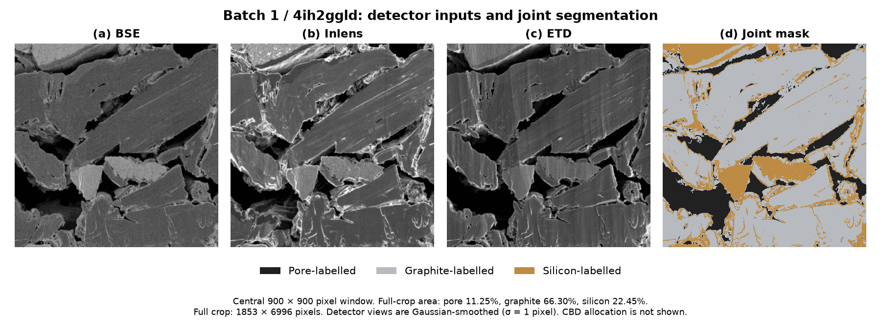
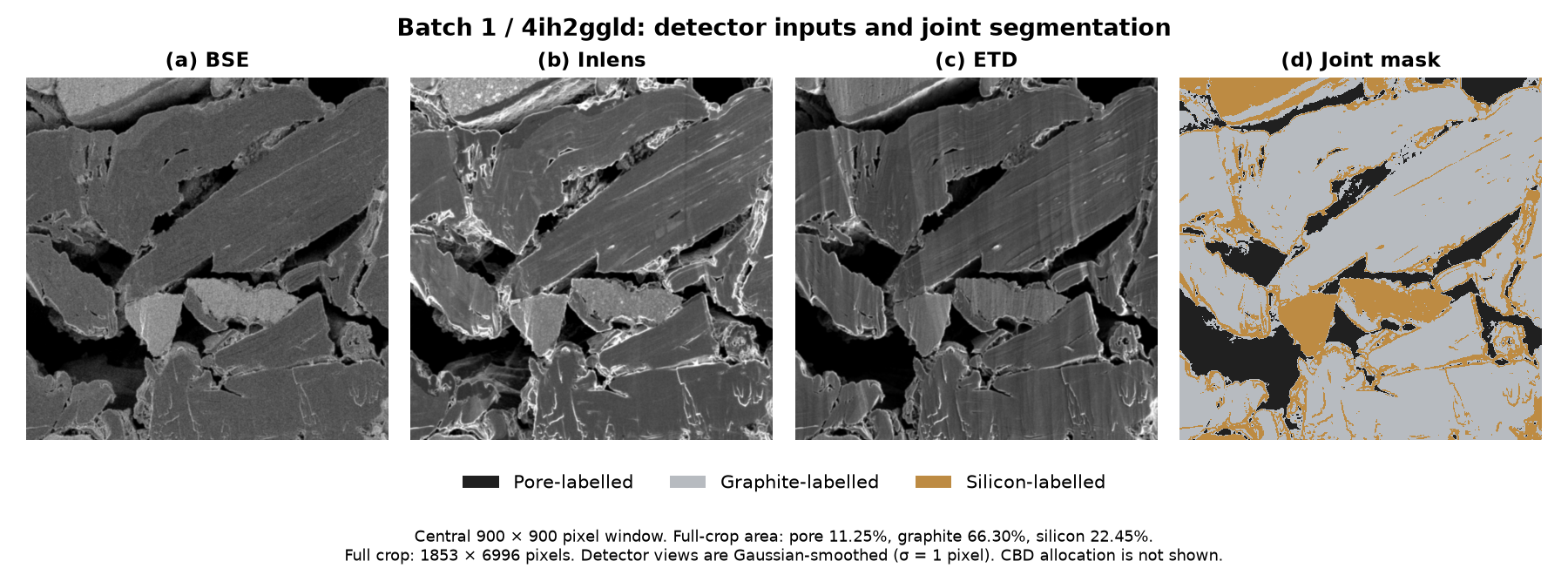
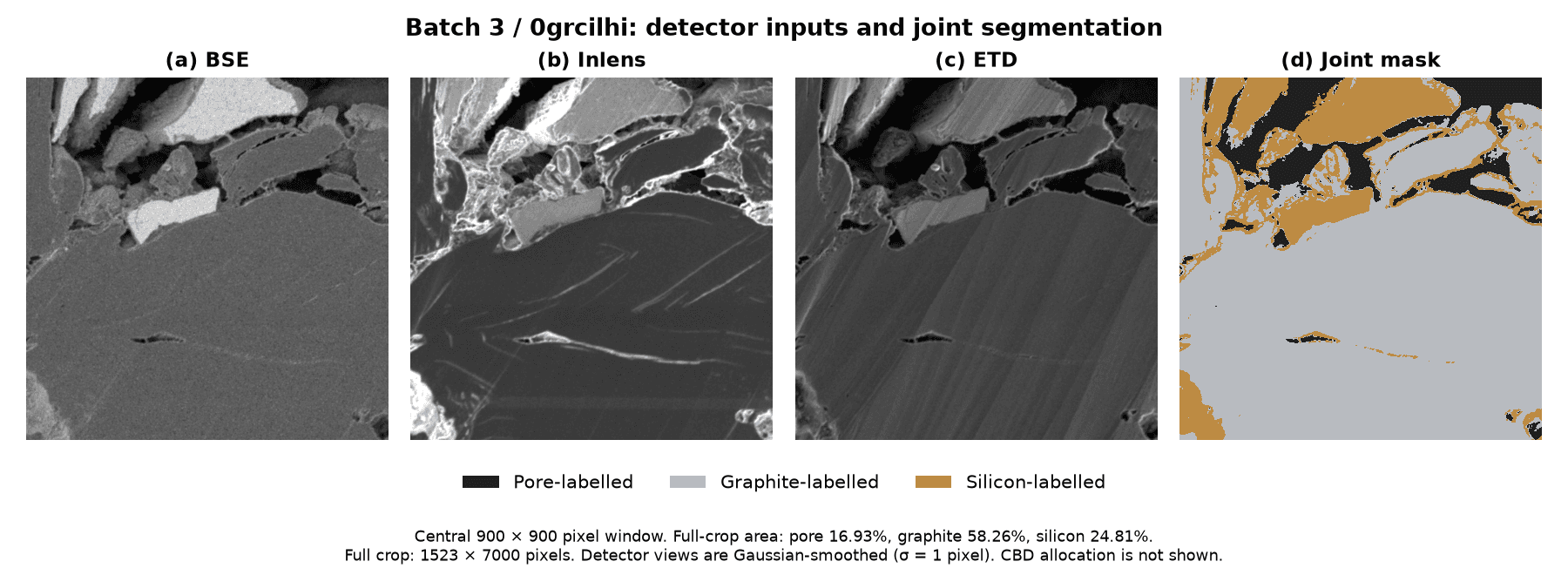
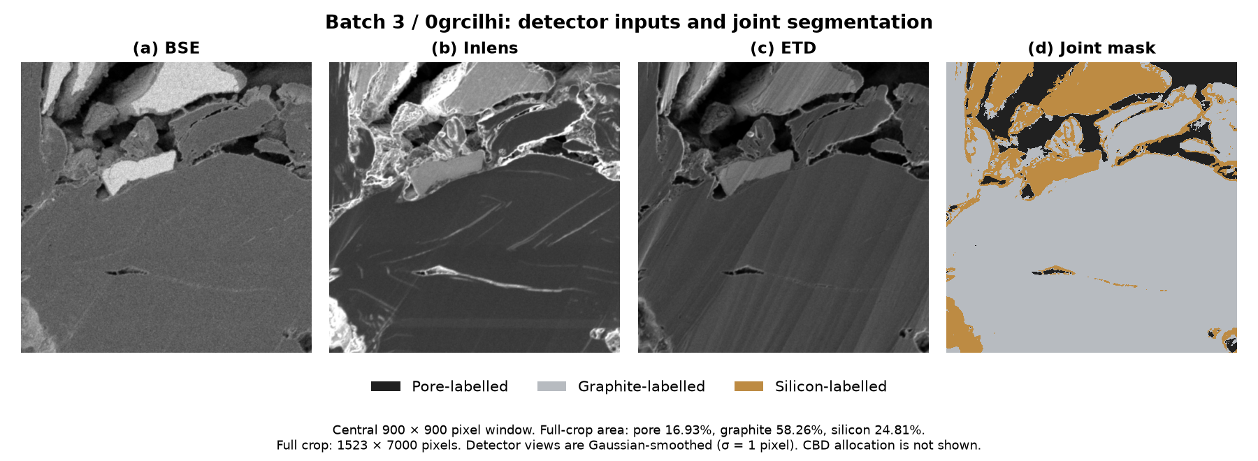
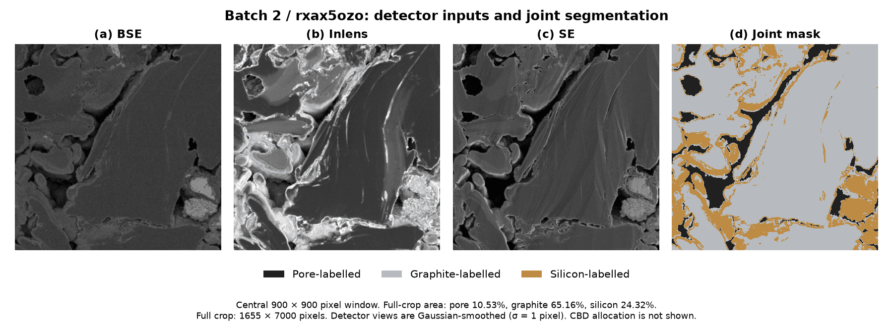
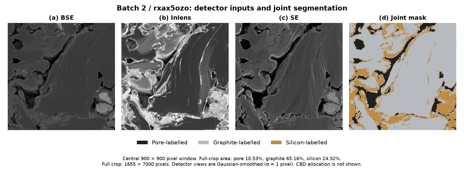
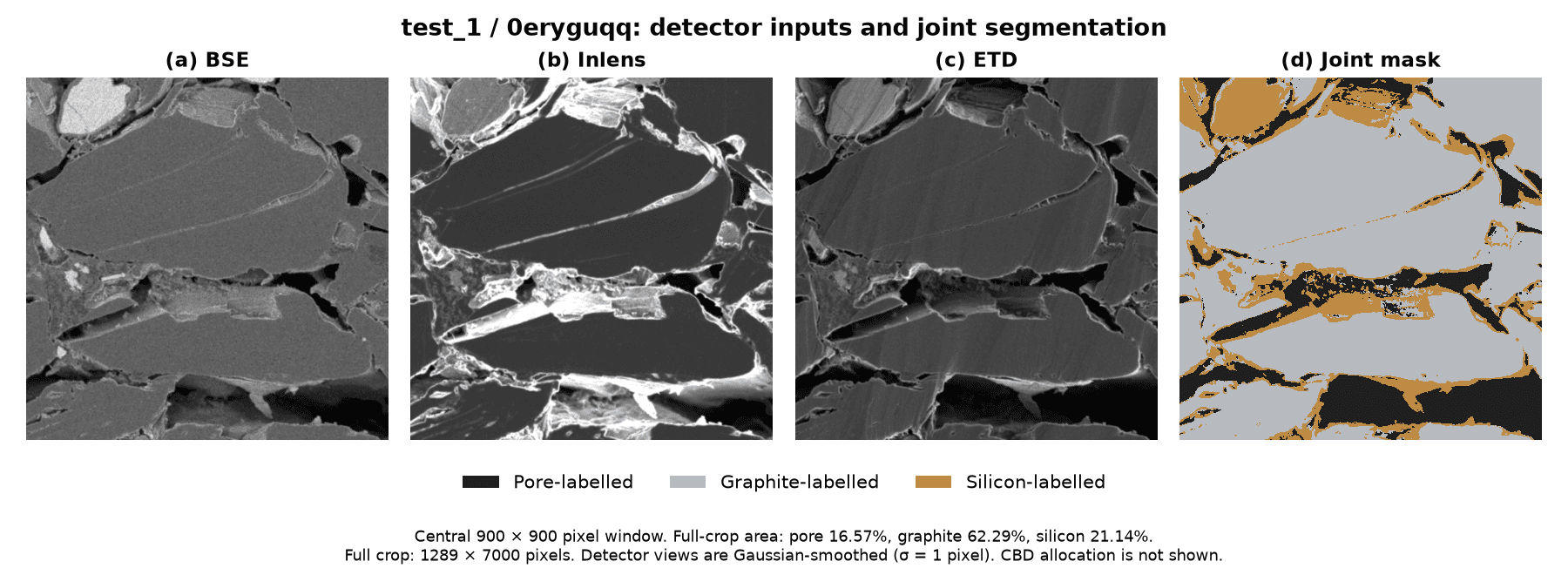
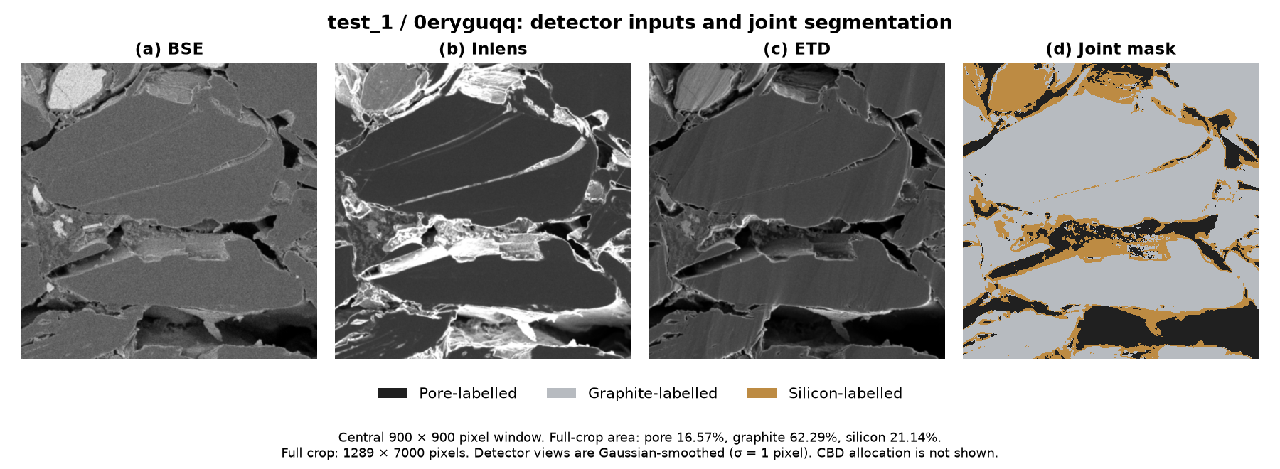
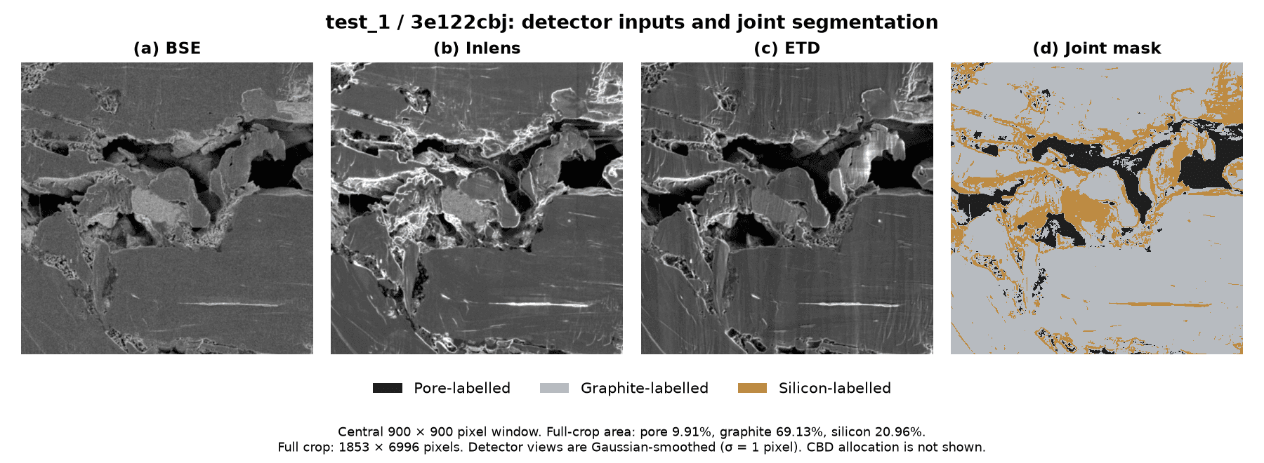
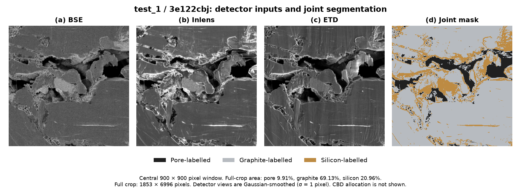
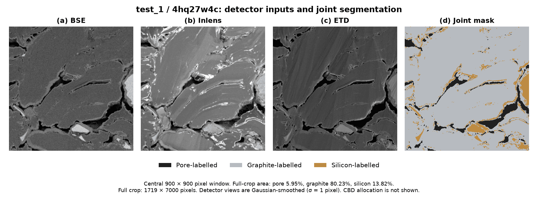
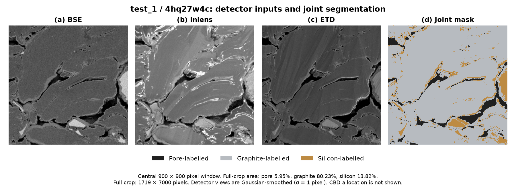
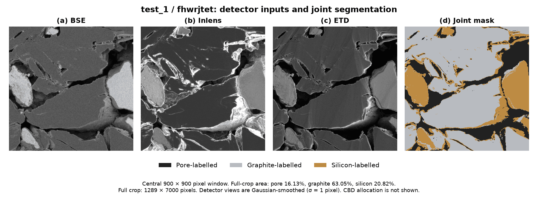
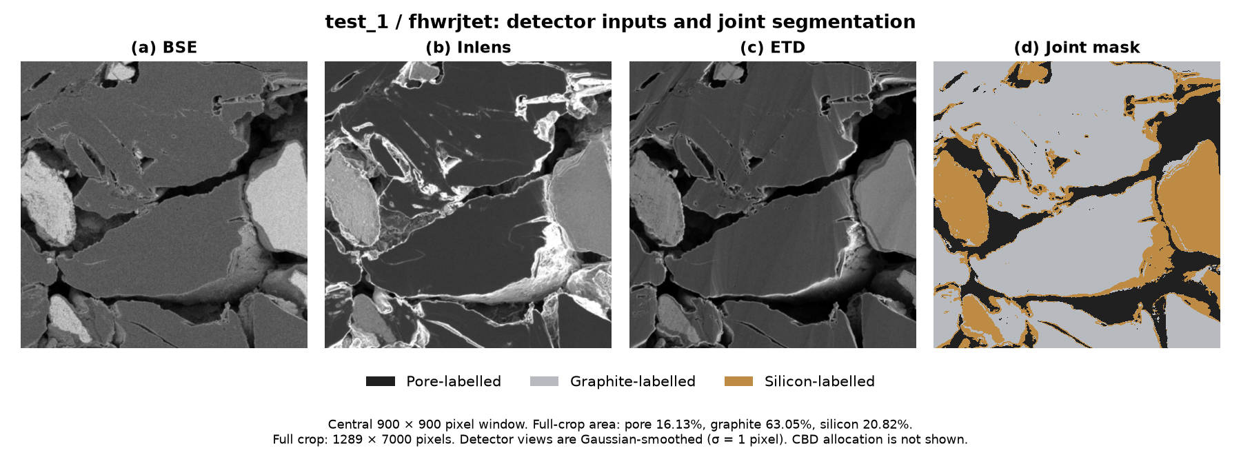
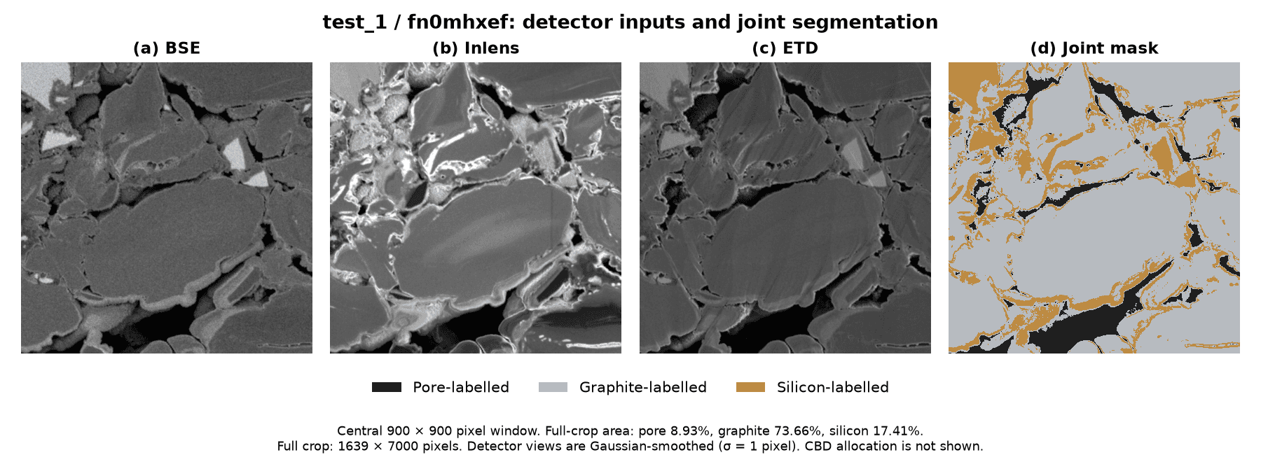
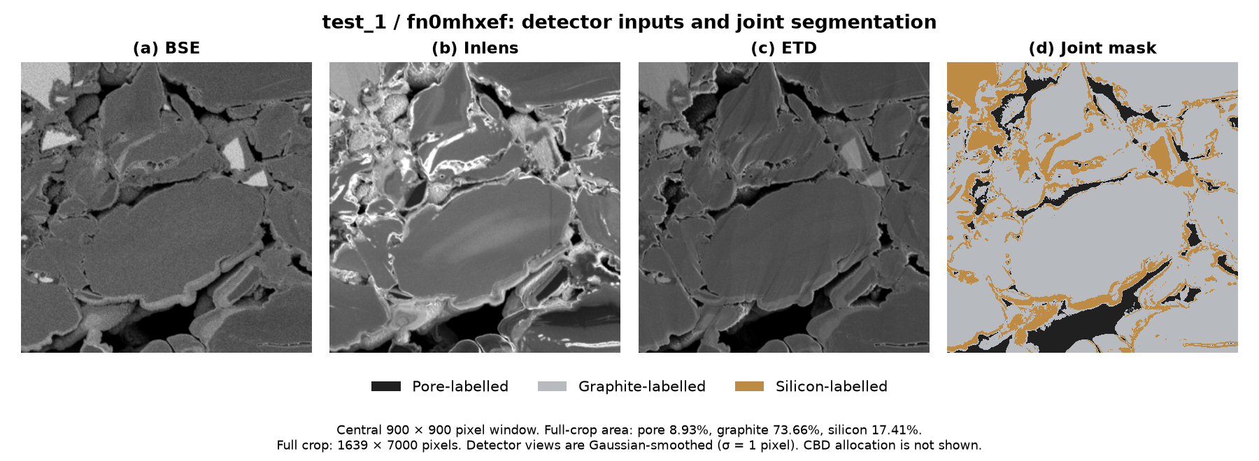
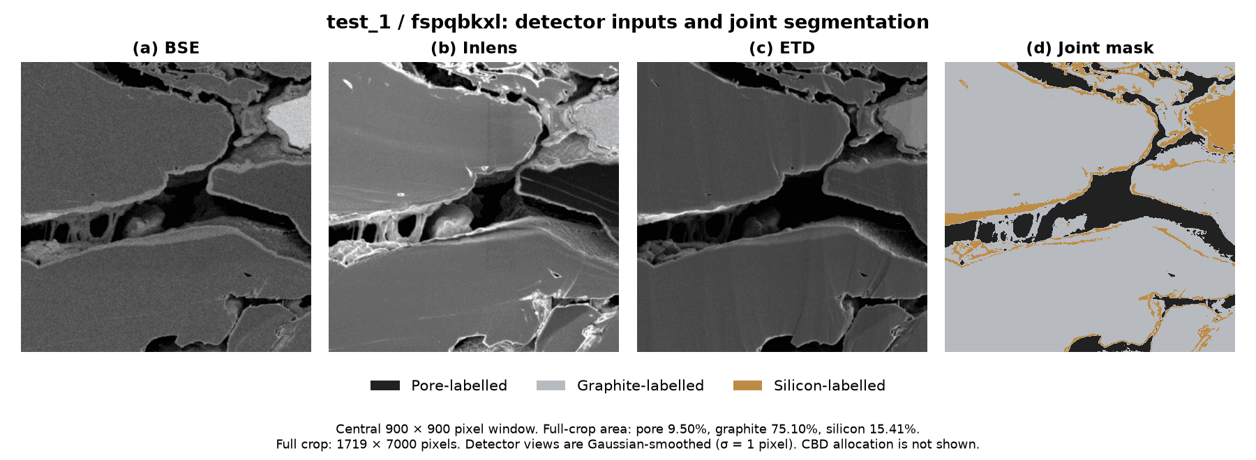
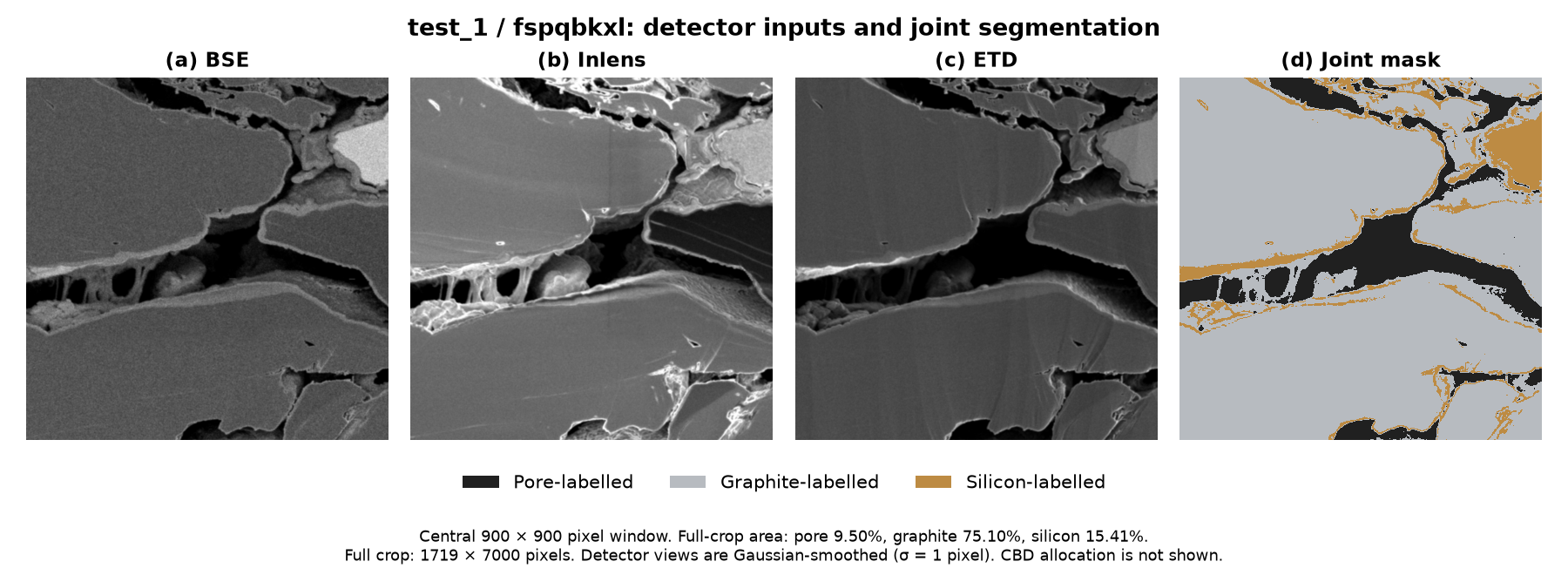
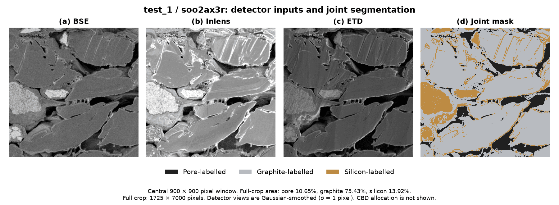
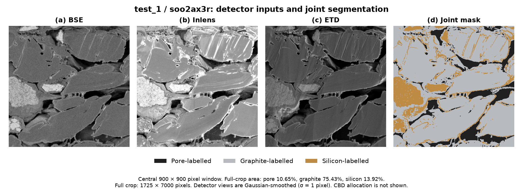
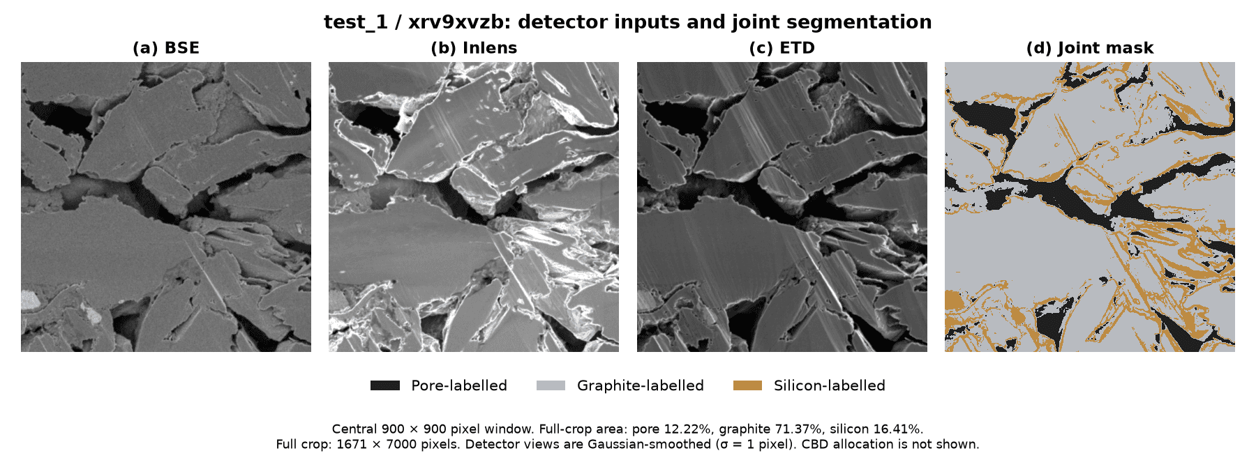
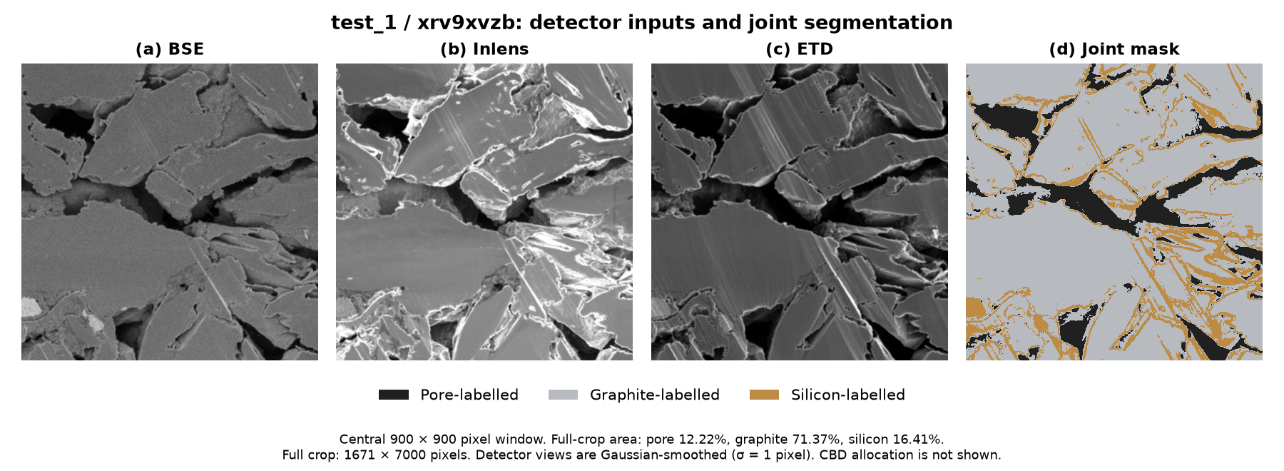
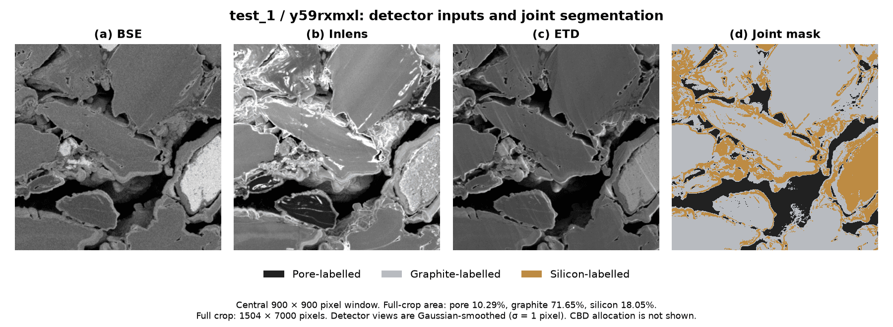
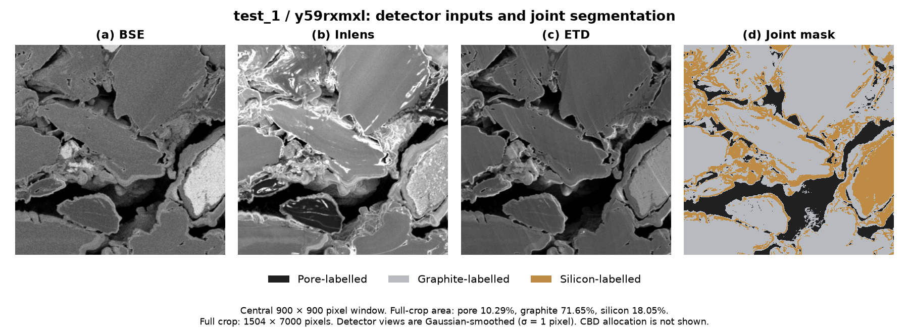
The method figures show four panels: smoothed BSE, Inlens, ETD/SE and the joint segmentation mask. They display matched central 900 × 900 pixel windows; measurements use the full crop. Additional rims and lines can enter the silicon-labelled class. These boundaries require validation before a segmented component can be treated as an individual particle. Inspect the segmentation.
Three-channel segmentation
Each pixel contributes separately standardized BSE, Inlens and ETD/SE intensities to KMeans. The channels are stacked, not averaged, and retain their original coordinates without automatic registration.
The first three panels show detector inputs after Gaussian smoothing (σ = 1 pixel); the fourth shows their joint segmentation. All panels display the same central 900 × 900 pixel window. Percentages use the whole crop, which retains the central 80% of image height. The separate CBD median allocation is not shown.
Inspect at full resolution: Fig. 1. Batch 1, sample 4ih2ggld
Scroll within the image to inspect details.
Fig. 1. Batch 1, sample 4ih2ggld. Detector inputs and the saved joint segmentation. The third detector is ETD. Silicon-labelled mask boundaries remain provisional.
Additional known samples
Batch 3, sample 0grcilhi
Inspect at full resolution: Fig. 2. Batch 3, sample 0grcilhi
Scroll within the image to inspect details.
Fig. 2. Batch 3, sample 0grcilhi. Detector inputs and the saved joint segmentation. The third detector is ETD. Silicon-labelled mask boundaries remain provisional.
Batch 2, sample rxax5ozo
Inspect at full resolution: Batch 2, sample rxax5ozo
Scroll within the image to inspect details.
Batch 2, sample rxax5ozo. Detector inputs and the saved joint segmentation. The third detector is SE. Silicon-labelled mask boundaries remain provisional.
Full test set (9 samples)
test_1, sample 0eryguqq
Inspect at full resolution: test_1, sample 0eryguqq
Scroll within the image to inspect details.
test_1, sample 0eryguqq. Detector inputs and the saved joint segmentation. The third detector is ETD. Silicon-labelled mask boundaries remain provisional.
test_1, sample 3e122cbj
Inspect at full resolution: test_1, sample 3e122cbj
Scroll within the image to inspect details.
test_1, sample 3e122cbj. Detector inputs and the saved joint segmentation. The third detector is ETD. Silicon-labelled mask boundaries remain provisional.
test_1, sample 4hq27w4c
Inspect at full resolution: test_1, sample 4hq27w4c
Scroll within the image to inspect details.
test_1, sample 4hq27w4c. Detector inputs and the saved joint segmentation. The third detector is ETD. Silicon-labelled mask boundaries remain provisional.
test_1, sample fhwrjtet
Inspect at full resolution: test_1, sample fhwrjtet
Scroll within the image to inspect details.
test_1, sample fhwrjtet. Detector inputs and the saved joint segmentation. The third detector is ETD. Silicon-labelled mask boundaries remain provisional.
test_1, sample fn0mhxef
Inspect at full resolution: test_1, sample fn0mhxef
Scroll within the image to inspect details.
test_1, sample fn0mhxef. Detector inputs and the saved joint segmentation. The third detector is ETD. Silicon-labelled mask boundaries remain provisional.
test_1, sample fspqbkxl
Inspect at full resolution: test_1, sample fspqbkxl
Scroll within the image to inspect details.
test_1, sample fspqbkxl. Detector inputs and the saved joint segmentation. The third detector is ETD. Silicon-labelled mask boundaries remain provisional.
test_1, sample soo2ax3r
Inspect at full resolution: test_1, sample soo2ax3r
Scroll within the image to inspect details.
test_1, sample soo2ax3r. Detector inputs and the saved joint segmentation. The third detector is ETD. Silicon-labelled mask boundaries remain provisional.
test_1, sample xrv9xvzb
Inspect at full resolution: test_1, sample xrv9xvzb
Scroll within the image to inspect details.
test_1, sample xrv9xvzb. Detector inputs and the saved joint segmentation. The third detector is ETD. Silicon-labelled mask boundaries remain provisional.
test_1, sample y59rxmxl
Inspect at full resolution: test_1, sample y59rxmxl
Scroll within the image to inspect details.
test_1, sample y59rxmxl. Detector inputs and the saved joint segmentation. The third detector is ETD. Silicon-labelled mask boundaries remain provisional.
Batch 3, sample 0grcilhi, using the combined three-detector segmentation. Descriptors retain their measured units; porosity uncertainty accompanies the vector separately. The saved record has 14 fields.Physical descriptor definitions (13)
The 13 physical descriptors in vector order. Example: Batch 3, sample 0grcilhi, from the saved measurements. Porosity uncertainty is defined separately below.
Physical descriptor
Value
Calculation
Pore area fraction%
16.93
Pore-labelled area / image area × 100. Describes the area assigned to voids.Calculation
Graphite-labelled area fraction%
58.26
Graphite-labelled area / image area × 100. Describes the assigned active-material fraction.Calculation
Carbon-binder allocation%
8.47
Pore-mask pixels above the median Inlens intensity / analysed area × 100. This heuristic assigns approximately half the pore area to CBD.Calculation
Silicon-labelled region area fraction%
24.81
Silicon-labelled area / image area × 100. Describes bright regions; their chemistry is not established by this value.Calculation
Characteristic length scaleµm
2.817
ImageRep integral_range × 0.025 µm/pixel, calculated from the binary pore mask. Describes the spatial correlation scale.Calculation
Vertical pore chord lengthµm
0.640
Mean uninterrupted pore run along image y, sampling every 40th column at 0.025 µm/pixel. A 2D chord, not a 3D throat width.Calculation
Horizontal pore chord lengthµm
0.770
Mean uninterrupted pore run along image x, sampling every 40th row at 0.025 µm/pixel.Calculation
Mean ellipse major axis / max(minor axis, 1 pixel), excluding zero minor axes. Calculated on silicon-labelled components of at least 10 pixels.Calculation
Silicon-labelled region diameter D10µm
0.098
10th percentile of area-equivalent diameter, d = s√(4A/π), where A is pixel area and s = 0.025 µm/pixel, for silicon-labelled components of at least 10 pixels. Each component has equal weight.Calculation
Silicon-labelled region diameter D50µm
0.174
Median area-equivalent diameter of the same silicon-labelled components. Connected regions can merge multiple particles; no particle separation is applied.Calculation
Silicon-labelled region diameter D90µm
0.607
90th percentile of the same unweighted silicon-component diameter distribution. Describes its larger objects.Calculation
Silicon-labelled region spatial variationpercentage points
6.16
Population standard deviation of silicon-labelled area percentages across a 4 × 4 grid. Describes local variation, not count variance / mean.Calculation
Porosity uncertainty
ImageRep estimates an absolute porosity error with confidence 0.95 and target error 0.05. Multiplying its returned absolute error by 100 gives the interval half-width in percentage points, stored as porosity_ci95_pct.
The interval estimates how representative the image is of bulk porosity. Dahari et al. (2025) provide the calculation. Measurement-error models such as Kelly (2007) treat uncertainty separately from observed values. Storing an interval alongside the descriptors does not by itself make a predictive model uncertainty-aware.
A smaller interval indicates a more precise porosity estimate under this model. It does not indicate a better material. The estimate is conditional on the pore mask and does not include segmentation or phase-assignment error.
Call ImageRep as make_error_prediction(pore_mask.astype(int), confidence=0.95, target_error=0.05). Its spatial-correlation model returns integral_range and abs_err; export these as integral_range × s and abs_err × 100. The implementation uses periodic FFT two-point correlation and includes its model-error correction. This is a correlation-based calculation.
target_error=0.05 is a relative error target, not a requirement that every interval equal ±5%. The interval estimates image representativity conditional on the segmentation and excludes phase-assignment error. A failed or nonfinite calculation stops extraction. ImageRep call; Dahari et al..
Pore chords and silicon-region geometry
Pad each sampled binary scan with zeros and pair positive and negative transitions; end − start gives the pore run length in pixels. Runs truncated by the crop boundary are included. Empty chord lists return zero, and anisotropy returns one if the vertical mean is zero. Horizontal and vertical refer to image axes; interpreting them as electrode directions requires known specimen orientation. These are two-dimensional chords, not three-dimensional pore throats or tortuosity. Chord calculation.
Label silicon-mask components using skimage.measure.label and measure them with regionprops. Retain components of at least 10 pixels. Diameter percentiles give equal weight to each retained component; no watershed separation or volume weighting is applied. Aspect ratios exclude zero minor axes and use a one-pixel minimum denominator. Empty diameter lists return zero and an empty aspect-ratio list returns one. Review these fallback values when interpreting a sample. Component calculation.
For spatial variation, np.array_split divides the silicon mask into 4 × 4 tiles. Calculate silicon coverage as a percentage within each tile, then use np.std(tile_percentages, ddof=0). This measures local area-fraction variation in percentage points, not a validated mixing or processing defect. Spatial calculation.
From measurements to batch comparisons
The assignment rule uses 13 of the 14 saved fields: it includes porosity uncertainty and excludes D10. These inputs differ from the 13 physical descriptors shown above. Each input is scaled by its standard deviation across the known crops, and the nearest batch mean determines the assignment.
Confidence bands use the fraction of correct predictions for that batch in leave-one-crop-out validation. They describe the rule’s observed reliability for a predicted batch, not the probability that an individual image is correctly assigned.
Batch assignment and confidence calculation
Nearest-batch assignment
The fixed classifier uses 13 assignment inputs: all 14 saved fields except D10. This is different from the 13 physical descriptors: it includes porosity uncertainty and excludes D10. The inputs retain correlated phase fractions, the CBD allocation and derived chord anisotropy; equal numerical weights do not make them independent physical evidence.
Fit one mean vector per known batch and calculate each input's sample standard deviation across all 31 known crops (ddof=1). Assign each test vector to the batch with the smallest root-mean-square standardized distance:
db=131j=1∑13(sjxj−xˉbj)2.
Known and test vectors must use the same three-detector segmentation. Scaling and batch means use known crops only; no test label enters fitting. An exact distance tie selects the first batch in the fixed order Batch 1, Batch 2, Batch 3. The rule identifies the closest known batch mean, not manufacturing equivalence. Assignment calculation.
For the website comparison, the relative similarity share is (1/db)/∑k(1/dk). These inverse-distance scores sum to 100% across the three batches. Equal distances give one third each; zero-distance matches share all the weight equally. All cells use one fixed numerical colour scale: red at zero, orange at one sixth, pale green at one third and dark green at 100%. Separate green, orange and red text annotations identify first, second and third rank. Outlined cells identify supplied organiser labels, independently of the predicted assignment. This display transformation preserves the nearest-mean assignment and is not a calibrated probability or validation confidence.
Assignment validation and confidence
Leave out one known crop, refit scaling and batch means on the other 30, then classify the omitted crop. Repeat for all 31 crops. The fixed rule correctly assigns 18 of 31 crops (58.1% accuracy; 49.3% balanced accuracy). For each predicted batch, divide correct assignments by all assignments to that batch:
Predicted batch
Correct / predicted
Observed validation rate
Confidence band
Batch 1
3 / 6
50.0%
Medium
Batch 2
2 / 10
20.0%
Low
Batch 3
13 / 15
86.7%
High
The reporting bands are High above 70%, Medium from 50% to 70% inclusive, and Low below 50%. They summarize class-level observed precision, not calibrated probabilities for individual images. Images assigned to the same batch share the same rate. Rates depend on the validation class composition and small sample counts.
Distance margins, agreement across 31 crop-omission refits and the assigned class's empirical distance envelope are retained as diagnostics. They do not change these reporting bands. Validation calculation; reporting thresholds.
The organisers describe crops from approximately 15 source electrode images, arranged into batches. A crop-to-parent mapping has not been established for this analysis, so crop-level validation may be optimistic. Future validation should hold out entire source images when that mapping is known.
Supplied labels identify 3e122cbj as Batch 2, fn0mhxef as Batch 1 and xrv9xvzb as Batch 3. The classifier assigns them to Batches 1, 2 and 3 respectively. These labels were available before the complete test evaluation and were not used to fit the classifier or calculate its confidence rates. Labels for the other six images have not been supplied. Batch assignment and its confidence band do not establish manufacturing acceptance.
Feature extraction code (Python)
The executed script for detector preparation, joint segmentation and physical measurements. The reported vectors use its stacked_three_channel output.
1#!/usr/bin/env python3
2"""Separate three-detector segmentation experiment; original exports are read-only."""
3from __future__ import annotations
45import argparse
6import csv
7import hashlib
8import json
9from pathlib import Path
10import platform
11import shutil
12import subprocess
13import sys
1415import matplotlib
16matplotlib.use("Agg")
17import matplotlib.pyplot as plt
18from matplotlib.colors import ListedColormap
19from matplotlib.patches import Patch
20import numpy as np
21from PIL import Image
22import sklearn
23import scipy
24import skimage
25import PIL
26from sklearn.cluster import KMeans
27from skimage.filters import gaussian, threshold_multiotsu
28from skimage.measure import label, regionprops
29from threadpoolctl import threadpool_limits
3031PORTAL_ROOT = Path(__file__).resolve().parents[1]
32ROOT = PORTAL_ROOT.parent
33sys.path.insert(0, str(PORTAL_ROOT / "scripts"))
34from extract_physical_features import FEATURE_COLUMNS, load_imagerep
35from compare_physical_batches import FEATURES
3637PIXEL_SIZE = .025
38VARIANTS = ["original_bse_otsu", "bse_kmeans_control", "stacked_three_channel"]
39PHASES = ["Pore-labelled", "Graphite-labelled", "Silicon-labelled"]
40COLOURS = ["#202020", "#b7bbc0", "#bd8b43"]
414243def digest(path):
44 return hashlib.sha256(Path(path).read_bytes()).hexdigest()
454647def inventory(data_dir, batch_names=None):
48 rows = []
49 for batch in batch_names or ["Batch_1", "Batch_2", "Batch_3", "test_1"]:
50 files = sorted((data_dir / batch).glob("img_*_BSE.tif"))
51 if not files:
52 raise ValueError(f"No BSE images in requested directory: {data_dir / batch}")
53 for bse in files:
54 sample = bse.stem.removeprefix("img_").removesuffix("_BSE")
55 inlens = bse.with_name(f"img_{sample}_Inlens.tif")
56 thirds = [bse.with_name(f"img_{sample}_{name}.tif") for name in ["ETD", "SE"]]
57 thirds = [p for p in thirds if p.exists()]
58 if not inlens.exists() or len(thirds) != 1:
59 raise ValueError(f"Expected BSE/Inlens and exactly one ETD or SE file: {sample}")
60 rows.append({"sample_id": sample, "batch": batch, "paths": [bse, inlens, thirds[0]],
61 "third_channel": thirds[0].stem.rsplit("_", 1)[1]})
62 if not rows:
63 raise ValueError("No samples found")
64 return rows
656667def load_channels(paths):
68 images, shapes = [], []
69 for path in paths:
70 with Image.open(path) as im:
71 raw = np.array(im)
72 if raw.ndim == 3:
73 raw = raw[:, :, 0]
74 if raw.ndim != 2:
75 raise ValueError(f"Expected a 2D intensity image: {path}")
76 shapes.append(raw.shape)
77 h = raw.shape[0]
78 images.append(gaussian(raw[int(.1*h):int(.9*h), :], sigma=1.0, preserve_range=True))
79 if len(set(shapes)) != 1:
80 raise ValueError("Channels have different pixel grids; no automatic resize or registration is performed")
81 return images, shapes[0]
828384def otsu_mask(bse):
85 low, high = threshold_multiotsu(bse, classes=3)
86 labels = np.zeros(bse.shape, dtype=np.uint8)
87 labels[bse >= low] = 1
88 labels[bse >= high] = 2
89 return labels, [float(low), float(high)]
909192def clustered_mask(channels, original, seed=42, max_pixels=100_000):
93 means = np.array([im.mean() for im in channels])
94 scales = np.array([im.std(ddof=0) for im in channels])
95 if not np.isfinite(scales).all() or np.any(scales <= 0):
96 raise ValueError("A detector image is constant or nonfinite")
97 flat = [im.ravel() for im in channels]
98 sampled_indices = np.random.default_rng(seed).choice(original.size, min(max_pixels, original.size), replace=False)
99 sampled = (np.column_stack([im[sampled_indices] for im in flat]) - means) / scales
100 sampled_labels = original.ravel()[sampled_indices]
101 if set(sampled_labels) != {0, 1, 2}:
102 raise ValueError("The sampled pixels do not contain all three initial BSE classes")
103 initial = np.array([sampled[sampled_labels == phase].mean(axis=0) for phase in range(3)])
104 model = KMeans(n_clusters=3, init=initial, n_init=1, random_state=seed,
105 max_iter=300, tol=1e-4, algorithm="lloyd").fit(sampled)
106 if model.n_iter_ >= 300:
107 raise ValueError("Clustering reached the iteration limit")
108 if len(set(model.labels_)) != 3:
109 raise ValueError("Clustering did not retain three distinct classes")
110 # Map joint clusters to the same intensity-based interpretation as the original.
111 order = np.argsort(model.cluster_centers_[:, 0], kind="stable")
112 mapping = np.empty(3, dtype=np.uint8)
113 mapping[order] = np.arange(3)
114 labels = np.empty(original.size, dtype=np.uint8)
115 for start in range(0, labels.size, 250_000):
116 end = min(start + 250_000, labels.size)
117 pixels = (np.column_stack([im[start:end] for im in flat]) - means) / scales
118 labels[start:end] = mapping[model.predict(pixels)]
119 return labels.reshape(original.shape), {
120 "channel_means": means.tolist(), "channel_population_sd": scales.tolist(),
121 "initial_normalised_centres_in_original_phase_order": initial.tolist(),
122 "normalised_cluster_centres_in_phase_order": model.cluster_centers_[order].tolist(),
123 "raw_cluster_centres_in_phase_order": (model.cluster_centers_[order] * scales + means).tolist(),
124 "sampled_pixels": len(sampled_indices), "seed": seed, "iterations": int(model.n_iter_),
125 "normalisation": "Per-image mean and population SD; each included channel has equal weight",
126 "initialisation": "Means of sampled pixels in the original three BSE Multi-Otsu masks",
127 "phase_mapping": "Increasing BSE cluster-centre intensity: pore, graphite, silicon",
128 }
129130131def measure_masks(labels, inlens, core):
132 """Original downstream calculations, with the segmentation masks as inputs."""
133 pore, matrix, silicon = labels == 0, labels == 1, labels == 2
134 if not 0 < pore.mean() < 1:
135 raise ValueError("Pore mask cannot be empty or fill the image")
136 median = np.median(inlens[pore])
137 cbd = pore & (inlens > median)
138 uncertainty = core.make_error_prediction(pore.astype(int), confidence=.95, target_error=.05)
139 chords = []
140 for axis in ["y", "x"]:
141 lines = (pore[:, col] for col in range(0, pore.shape[1], 40)) if axis == "y" else (pore[row, :] for row in range(0, pore.shape[0], 40))
142 lengths = []
143 for line in lines:
144 diffs = np.diff(np.concatenate(([0], line.astype(int), [0])))
145 starts, ends = np.where(diffs == 1)[0], np.where(diffs == -1)[0]
146 lengths.extend((ends - starts) * PIXEL_SIZE)
147 chords.append(float(np.mean(lengths)) if lengths else 0.0)
148 ly, lx = chords
149 props = [p for p in regionprops(label(silicon)) if p.area >= 10]
150 diameters = [p.equivalent_diameter_area * PIXEL_SIZE for p in props]
151 ratios = [p.axis_major_length / max(p.axis_minor_length, 1) for p in props if p.axis_minor_length > 0]
152 d10, d50, d90 = np.percentile(diameters, [10, 50, 90]) if diameters else [0., 0., 0.]
153 tiles = [100*np.mean(tile) for band in np.array_split(silicon, 4, axis=0) for tile in np.array_split(band, 4, axis=1)]
154 values = [100*float(pore.mean()), 100*float(uncertainty["abs_err"]),
155 100*float(matrix.mean()), 100*float(cbd.mean()), 100*float(silicon.mean()),
156 PIXEL_SIZE*float(uncertainty["integral_range"]), ly, lx, lx/ly if ly > 0 else 1.,
157 float(np.mean(ratios)) if ratios else 1., float(d10), float(d50), float(d90), float(np.std(tiles, ddof=0))]
158 if not np.isfinite(values).all():
159 raise ValueError("A physical calculation returned a nonfinite value")
160 return dict(zip(FEATURE_COLUMNS, values))
161162163def saved_features():
164 result = {}
165 aliases = {f["key"]: f["raw_key"] for f in FEATURES}
166 aliases["porosity_ci95_pct"] = "ci95_abs_pct"
167 for filename, canonical in [("qc_dataset_features.csv", False), ("test_1_physical_features.csv", True)]:
168 with (PORTAL_ROOT / "public" / filename).open(newline="") as handle:
169 for row in csv.DictReader(handle):
170 result[row["sample_id"]] = {key: float(row[key if canonical else aliases[key]]) for key in FEATURE_COLUMNS}
171 return result
172173174def mask_comparison(original, candidate):
175 output = {"changed_pixel_fraction": float(np.mean(original != candidate))}
176 for k, name in enumerate(["pore", "graphite", "silicon"]):
177 a, b = original == k, candidate == k
178 output[name + "_iou"] = float(np.sum(a & b) / np.sum(a | b))
179 output[name + "_dice"] = float(2 * np.sum(a & b) / (np.sum(a) + np.sum(b)))
180 output[name + "_changed_pixel_fraction"] = float(np.mean(a != b))
181 return output
182183184def draw_masks(row, channels, masks, measurements, output):
185 # Display a fixed centre window; segmentation and measurements use the full crop.
186 h, w = channels[0].shape
187 size = min(900, h, w)
188 y, x = (h-size)//2, (w-size)//2
189 view = (slice(y, y+size), slice(x, x+size))
190 fig, axes = plt.subplots(2, 3, figsize=(12, 9.8))
191 for ax, im, name in zip(axes[0], channels, ["BSE", "Inlens", row["third_channel"]]):
192 ax.imshow(im[view], cmap="gray", vmin=float(im.min()), vmax=float(im.max()))
193 ax.set_title(name, fontweight="bold")
194 for ax, mask, variant, title in zip(axes[1], masks, VARIANTS,
195 ["Original BSE Multi-Otsu", "BSE-only clustering control", "Three-channel clustering"]):
196 value = measurements[variant]
197 ax.imshow(mask[view], cmap=ListedColormap(COLOURS), vmin=0, vmax=2, interpolation="nearest")
198 ax.set_title(f"{title}\nPore {value['porosity_pct']:.2f}%; silicon {value['inclusion_pct']:.2f}%", fontsize=11)
199 for ax in axes.flat:
200 ax.set_axis_off()
201 fig.suptitle(f"{row['batch']} / {row['sample_id']}: matched detector views and masks", fontsize=14, fontweight="bold")
202 fig.legend(handles=[Patch(facecolor=c, label=p) for c, p in zip(COLOURS, PHASES)],
203 loc="lower center", bbox_to_anchor=(.5, .055), ncol=3, frameon=False)
204 fig.text(.5, .022, f"Same central {size} × {size} pixel display window. Percentages use the entire {h} × {w} pixel crop.\nIntensity clusters are candidate phase masks; CBD median allocation is not shown.", ha="center", fontsize=9)
205 fig.subplots_adjust(left=.025, right=.975, top=.94, bottom=.13, wspace=.04, hspace=.12)
206 fig.savefig(output, dpi=150, facecolor="white")
207 plt.close(fig)
208209210def main():
211 parser = argparse.ArgumentParser(description=__doc__)
212 parser.add_argument("--data-dir", type=Path, default=ROOT / "data")
213 parser.add_argument("--run-dir", type=Path, required=True)
214 parser.add_argument("--imagerep-path", type=Path, default=ROOT / "ImageRep")
215 parser.add_argument("--batch-name", action="append", help="Folder under --data-dir; repeat to select several folders")
216 parser.add_argument("--sample-id", action="append", default=[])
217 args = parser.parse_args()
218 if args.run_dir.exists():
219 parser.error("Run directory already exists; choose a new directory")
220 rows = inventory(args.data_dir, args.batch_name)
221 if args.sample_id:
222 rows = [r for r in rows if r["sample_id"] in args.sample_id]
223 if set(args.sample_id) != {r["sample_id"] for r in rows}:
224 parser.error("Requested sample not found")
225 args.run_dir.mkdir(parents=True)
226 (args.run_dir / "figures").mkdir()
227 (args.run_dir / "masks").mkdir()
228 original_values = saved_features()
229 core = load_imagerep(args.imagerep_path)
230 source_files = [Path(__file__), PORTAL_ROOT / "scripts/extract_physical_features.py",
231 PORTAL_ROOT / "scripts/compare_physical_batches.py", Path(core.__file__)]
232 source_dir = args.run_dir / "source_snapshot"
233 source_dir.mkdir()
234 source_hashes = {str(p): digest(p) for p in source_files}
235 for path in source_files:
236 shutil.copy2(path, source_dir / path.name)
237 imagerep_revision = subprocess.check_output(["git", "-C", str(args.imagerep_path), "rev-parse", "HEAD"], text=True).strip()
238 records, features = [], []
239 for index, row in enumerate(rows):
240 print(f"[{index+1}/{len(rows)}] {row['batch']}/{row['sample_id']} ({row['third_channel']})", flush=True)
241 channels, native_shape = load_channels(row["paths"])
242 original, thresholds = otsu_mask(channels[0])
243 # Validate the unchanged downstream calculation against saved full precision.
244 baseline = measure_masks(original, channels[1], core)
245 saved = original_values.get(row["sample_id"])
246 errors = {key: abs(baseline[key] - saved[key]) for key in FEATURE_COLUMNS} if saved else None
247 if errors is not None and max(errors.values()) > 1e-10:
248 raise ValueError(f"Original-method reproduction failed for {row['sample_id']}: {errors}")
249 with threadpool_limits(limits=1):
250 bse, bse_fit = clustered_mask(channels[:1], original)
251 stacked, stack_fit = clustered_mask(channels, original)
252 masks = [original, bse, stacked]
253 measured = {VARIANTS[0]: baseline, VARIANTS[1]: measure_masks(bse, channels[1], core),
254 VARIANTS[2]: measure_masks(stacked, channels[1], core)}
255 for variant, mask in zip(VARIANTS, masks):
256 features.append({"batch": row["batch"], "sample_id": row["sample_id"],
257 "third_channel": row["third_channel"], "variant": variant, **measured[variant]})
258 Image.fromarray(mask).save(args.run_dir / "masks" / f"{row['sample_id']}_{variant}.png")
259 draw_masks(row, channels, masks, measured, args.run_dir / "figures" / f"{row['sample_id']}.png")
260 records.append({"batch": row["batch"], "sample_id": row["sample_id"], "third_channel": row["third_channel"],
261 "input_files": [{"path": str(p), "sha256": digest(p)} for p in row["paths"]],
262 "native_shape": list(native_shape), "crop_shape": list(original.shape),
263 "original_thresholds": thresholds, "original_max_absolute_feature_error": max(errors.values()) if errors is not None else None,
264 "original_verification": "Compared with saved values" if saved else "New sample; no previous export to compare",
265 "fits": {VARIANTS[1]: bse_fit, VARIANTS[2]: stack_fit}, "measurements": measured,
266 "agreement_with_original": {VARIANTS[1]: mask_comparison(original, bse), VARIANTS[2]: mask_comparison(original, stacked)},
267 "added_channel_effect": mask_comparison(bse, stacked)})
268 (args.run_dir / "progress.json").write_text(json.dumps(records, allow_nan=False) + "\n")
269 print(" pore fractions: " + ", ".join(f"{v}={measured[v]['porosity_pct']:.2f}%" for v in VARIANTS), flush=True)
270 with (args.run_dir / "features.csv").open("w", newline="") as handle:
271 writer = csv.DictWriter(handle, fieldnames=["batch", "sample_id", "third_channel", "variant", *FEATURE_COLUMNS])
272 writer.writeheader()
273 writer.writerows(features)
274 report = {"experiment": "Three-channel intensity segmentation v1", "status": "Exploratory side experiment; original results unchanged",
275 "method": {"pixel_size_um": PIXEL_SIZE, "crop": "central 80% rows, all columns", "gaussian_sigma_px": 1,
276 "third_channel": "ETD or SE, treated as the third detector at the user's direction",
277 "registration": "No registration or resampling; matched pixel grids assumed, separate alignment audit",
278 "clustering": "Three KMeans intensity classes; per-image channel z-scores; 100000 sampled pixels; BSE Multi-Otsu initial centres; seed42; n_init1",
279 "downstream": "Same 14 saved physical fields, including the separate heuristic Inlens median CBD allocation",
280 "silicon": "Bright phase identified as silicon by the user; intensity-derived boundaries still require validation",
281 "agreement": "Mask IoU, Dice and changed-pixel fractions measure agreement, not accuracy against ground truth",
282 "test_labels": "Not used in segmentation, measurement or settings"},
283 "script_sha256": digest(__file__), "original_extractor_sha256": digest(PORTAL_ROOT / "scripts/extract_physical_features.py"),
284 "source_hashes": source_hashes, "imagerep_revision": imagerep_revision,
285 "versions": {"python": platform.python_version(), "numpy": np.__version__, "sklearn": sklearn.__version__,
286 "scipy": scipy.__version__, "skimage": skimage.__version__, "pillow": PIL.__version__,
287 "matplotlib": matplotlib.__version__},
288 "samples": records}
289 (args.run_dir / "report.json").write_text(json.dumps(report, indent=2, allow_nan=False) + "\n")
290 print(f"Wrote {len(rows)} × 3 feature records to {args.run_dir}")
291292293if __name__ == "__main__":
294 main()
Batch assignment code (Python)
The executed assignment script. The reported confidence bands use the empirical_precision_v2 option specified in the protocol.
1#!/usr/bin/env python3
2"""Assign multichannel physical vectors with a fixed, transparent centroid rule.
34First run without --test-csv to freeze the method and evaluate known crops.
5Then supply --test-csv with the same output directory. No test labels are used.
6Confidence bands describe heuristic assignment support, never probabilities or
7manufacturing acceptance. All evaluation remains provisional at crop level.
8"""
9from __future__ import annotations
1011import argparse
12import csv
13from datetime import datetime, timezone
14import hashlib
15import json
16from pathlib import Path
17import platform
1819import numpy as np
202122CLASSES = ("Batch_1", "Batch_2", "Batch_3")
23VARIANT = "stacked_three_channel"
24FEATURES = (
25 ("porosity_pct", "Pore-labelled area fraction", "%"),
26 ("porosity_ci95_pct", "Porosity uncertainty half-width", "percentage points"),
27 ("active_material_pct", "Graphite-labelled area fraction", "%"),
28 ("cbd_pct", "Carbon-binder allocation", "%"),
29 ("inclusion_pct", "Silicon-labelled area fraction", "%"),
30 ("char_length_scale_cls_um", "Pore correlation length", "µm"),
31 ("throat_through_plane_ly_um", "Vertical pore chord", "µm"),
32 ("chord_in_plane_lx_um", "Horizontal pore chord", "µm"),
33 ("pore_anisotropy_ratio", "Horizontal/vertical pore chord ratio", "ratio"),
34 ("particle_aspect_ratio", "Silicon-labelled domain aspect ratio", "ratio"),
35 ("particle_d50_um", "Silicon-labelled domain diameter D50", "µm"),
36 ("particle_d90_um", "Silicon-labelled domain diameter D90", "µm"),
37 ("slurry_dispersion_index", "Silicon-labelled area spatial variation", "percentage points"),
38)
39KEYS = tuple(item[0] for item in FEATURES)
40# Fixed before inspecting the full test vectors. These are design choices,
41# not empirically calibrated probability cutoffs or optimized hyperparameters.
42THRESHOLDS = {
43 "High": {"oof_precision_min": 0.85, "oof_prediction_count_min": 5,
44 "relative_margin_min": 0.25, "leave_one_crop_out_agreement_min": 0.90},
45 "Medium": {"oof_precision_min": 0.60, "oof_prediction_count_min": 5,
46 "relative_margin_min": 0.10, "leave_one_crop_out_agreement_min": 0.75},
47}
48SUPPORT_QUANTILE = 0.95
49POLICIES = ("conservative_v1", "empirical_precision_v2")
50CONFIDENCE_POLICY_V2 = {
51 "requested_by": "User", "threshold_source": "Explicit user instruction; no outcome-based threshold search",
52 "revision_context": "Reporting bands revised after the v1 assignment summary. The fitted classifier, features and assignments are unchanged.",
53 "score": "100 * correctly assigned known crops / all known crops predicted as the assigned class in leave-one-crop-out evaluation",
54 "score_scope": "Class-level observed validation precision; not an individual calibrated probability",
55 "thresholds": {"High": "strictly greater than70%", "Medium": "50% through70%, inclusive", "Low": "below50%"},
56 "other_checks": "Distance margin, omission agreement and empirical support envelope remain diagnostics and do not change this user-defined band",
57}
58LIMITATIONS = [
59 "The ratings are heuristic assignment support, not calibrated probabilities.",
60 "Known crops may share original images; parent-image groups are unavailable. Leave-one-crop-out evaluation can therefore be optimistic.",
61 "Per-class precision estimates are based on few crop predictions and unknown test class proportions.",
62 "Thirteen equally standardized exported fields retain correlated and derived variables, including porosity uncertainty and the carbon-binder allocation. They are not thirteen independent physical mechanisms.",
63 "The support envelope is an empirical distance summary, not a conformal prediction region or a 95% probability statement.",
64 "Leave-one-crop-out agreement measures sensitivity to individual known crops, not correctness or uncertainty in phase boundaries.",
65 "Silicon-labelled mask boundaries remain unvalidated and can include rims or lines; pore chords do not establish three-dimensional transport.",
66 "Three earlier test identities have already been revealed. This is not an untouched external validation exercise; test labels are nevertheless excluded from fitting and confidence calculations.",
67 "Batch identity does not establish manufacturing quality. No accept or reject decision is produced.",
68]
697071def sha256(path):
72 return hashlib.sha256(Path(path).read_bytes()).hexdigest()
737475def canonical_hash(value):
76 return hashlib.sha256(json.dumps(value, sort_keys=True, separators=(",", ":"),
77 allow_nan=False).encode()).hexdigest()
787980def write_json(path, value):
81 Path(path).write_text(json.dumps(value, indent=2, allow_nan=False) + "\n")
828384def read_vectors(path, *, known):
85 """Read only the requested method and split; never read test-label columns."""
86 records = []
87 with Path(path).open(newline="", encoding="utf-8-sig") as handle:
88 reader = csv.DictReader(handle)
89 header = reader.fieldnames or []
90 required = {"batch", "sample_id", "variant", *KEYS}
91 if len(header) != len(set(header)) or not required.issubset(header):
92 raise ValueError("Unique CSV columns including batch, sample_id, variant and all13 fixed fields are required")
93 seen = set()
94 for row in reader:
95 if None in row or any(value is None for value in row.values()):
96 raise ValueError("Malformed CSV row")
97 if row["variant"] != VARIANT:
98 continue
99 batch = row["batch"].strip()
100 if known and batch not in CLASSES:
101 continue
102 if not known and batch in CLASSES:
103 raise ValueError("Test input includes known-batch rows; provide the separate test extraction")
104 sample = row["sample_id"].strip()
105 if not sample or sample in seen:
106 raise ValueError("Sample IDs must be nonempty and unique within the selected variant")
107 seen.add(sample)
108 values = [float(row[key]) for key in KEYS]
109 if not np.isfinite(values).all():
110 raise ValueError(f"Nonfinite vector: {sample}")
111 records.append({"sample_id": sample, "batch": batch,
112 "third_channel": row.get("third_channel", ""), "values": values})
113 if not records:
114 raise ValueError("No vectors for the selected method and split")
115 if known and (len(records) != 31 or {label: sum(r["batch"] == label for r in records)
116 for label in CLASSES} != {"Batch_1": 7, "Batch_2": 7, "Batch_3": 17}):
117 raise ValueError("This frozen study requires the original31 known crops (7,7,17)")
118 return records
119120121def fit_rule(x, y):
122 mean = x.mean(axis=0)
123 scale = x.std(axis=0, ddof=1)
124 if not np.isfinite(scale).all() or np.any(scale <= 0):
125 raise ValueError("All13 frozen fields must have positive training sample SD")
126 centers = np.stack([x[y == label].mean(axis=0) for label in CLASSES])
127 return {"mean": mean, "scale": scale, "centroids": centers}
128129130def distances(rule, x):
131 x = np.atleast_2d(x)
132 squared = ((x[:, None, :] - rule["centroids"][None, :, :]) / rule["scale"]) ** 2
133 return np.sqrt(squared.mean(axis=2)), squared
134135136def relative_margin(values):
137 order = np.argsort(values, kind="stable")
138 best, runner = order[:2]
139 # Equal zero distances are an exact tie, not maximal alignment.
140 margin = float((values[runner] - values[best]) / values[runner]) if values[runner] > 0 else 0.0
141 return int(best), int(runner), margin
142143144def wilson_interval(correct, total):
145 """Descriptive binomial interval only; shared parent crops violate its model."""
146 if total == 0:
147 return [None, None]
148 z = 1.959963984540054
149 p = correct / total
150 denominator = 1 + z * z / total
151 center = (p + z * z / (2 * total)) / denominator
152 half = z * np.sqrt(p * (1 - p) / total + z * z / (4 * total * total)) / denominator
153 return [float(center - half), float(center + half)]
154155156def evaluate_known(records):
157 x = np.array([r["values"] for r in records])
158 y = np.array([r["batch"] for r in records])
159 rows, omission_rules = [], []
160 matrix = np.zeros((3, 3), dtype=int)
161 for i, record in enumerate(records):
162 keep = np.arange(len(records)) != i
163 rule = fit_rule(x[keep], y[keep])
164 omission_rules.append(rule)
165 ds, _ = distances(rule, x[i])
166 best, runner, margin = relative_margin(ds[0])
167 actual = CLASSES.index(record["batch"])
168 matrix[actual, best] += 1
169 rows.append({"sample_id": record["sample_id"], "actual_batch": record["batch"],
170 "assigned_batch": CLASSES[best], "runner_up": CLASSES[runner],
171 "correct": best == actual, "relative_margin": margin,
172 "true_class_distance": float(ds[0, actual]),
173 "distances": dict(zip(CLASSES, ds[0].tolist()))})
174 per_class = {}
175 for j, label in enumerate(CLASSES):
176 n_predicted, n_actual, correct = int(matrix[:, j].sum()), int(matrix[j].sum()), int(matrix[j, j])
177 true_distances = [r["true_class_distance"] for r in rows if r["actual_batch"] == label]
178 per_class[label] = {"actual_crop_count": n_actual, "oof_prediction_count": n_predicted,
179 "oof_correct_predictions": correct,
180 "oof_precision": correct / n_predicted if n_predicted else None,
181 "oof_recall": correct / n_actual,
182 "descriptive_binomial_precision_interval95": wilson_interval(correct, n_predicted),
183 "true_class_loo_distance_quantile95": float(np.quantile(true_distances, SUPPORT_QUANTILE, method="linear")),
184 "true_class_loo_distances": true_distances}
185 evaluation = {"class_order": list(CLASSES), "confusion_matrix_actual_rows_predicted_columns": matrix.tolist(),
186 "correct": int(matrix.trace()), "crop_count": len(records),
187 "accuracy": float(matrix.trace() / len(records)),
188 "balanced_accuracy": float(np.mean(matrix.diagonal() / matrix.sum(axis=1))),
189 "per_class": per_class, "predictions": rows,
190 "precision_interval_note": "Wilson intervals assume independent Bernoulli outcomes; shown descriptively only because crop dependence is unresolved.",
191 "evaluation_scope": "Fixed-rule leave-one-known-crop-out; scaling and centroids refitted using the other30 crops in each fold."}
192 return evaluation, fit_rule(x, y), omission_rules
193194195def confidence_band(precision, count, margin, stability, within_support):
196 checks = {}
197 for name, thresholds in THRESHOLDS.items():
198 checks[name] = {
199 "class_oof_precision": precision is not None and precision >= thresholds["oof_precision_min"],
200 "class_oof_prediction_count": count >= thresholds["oof_prediction_count_min"],
201 "relative_margin": margin >= thresholds["relative_margin_min"],
202 "leave_one_crop_out_agreement": stability >= thresholds["leave_one_crop_out_agreement_min"],
203 "within_assigned_class_support": bool(within_support),
204 }
205 band = next((name for name in THRESHOLDS if all(checks[name].values())), "Low")
206 return band, checks
207208209def precision_rating(precision):
210 if precision is None:
211 return "Low"
212 return "High" if precision > 0.70 else "Medium" if precision >= 0.50 else "Low"
213214215def assign_tests(test, known, evaluation, rule, omission_rules, policy="conservative_v1"):
216 x = np.array([r["values"] for r in test])
217 known_x = np.array([r["values"] for r in known])
218 known_y = np.array([r["batch"] for r in known])
219 ds, squared = distances(rule, x)
220 omission_predictions = np.array([np.argmin(distances(r, x)[0], axis=1) for r in omission_rules])
221 assignments = []
222 for i, record in enumerate(test):
223 best, runner, margin = relative_margin(ds[i])
224 label = CLASSES[best]
225 validation = evaluation["per_class"][label]
226 stability = float(np.mean(omission_predictions[:, i] == best))
227 envelope = validation["true_class_loo_distance_quantile95"]
228 inside = bool(ds[i, best] <= envelope)
229 band, checks = confidence_band(validation["oof_precision"], validation["oof_prediction_count"], margin, stability, inside)
230 # The summed contributions equal runner-up squared RMS distance minus
231 # assigned squared RMS distance. Positive values favour the assignment.
232 support = (squared[i, runner] - squared[i, best]) / len(KEYS)
233 features = []
234 for j, (key, name, unit) in enumerate(FEATURES):
235 summaries = {}
236 for batch in CLASSES:
237 values = known_x[known_y == batch, j]
238 summaries[batch] = {"mean": float(values.mean()), "sample_sd": float(values.std(ddof=1)),
239 "min": float(values.min()), "max": float(values.max())}
240 features.append({"key": key, "label": name, "unit": unit, "value": record["values"][j],
241 "known_batches": summaries,
242 "assigned_minus_runner_squared_distance_support": float(support[j]),
243 "standardized_difference_from_assigned_mean": float((x[i, j] - rule["centroids"][best, j]) / rule["scale"][j]),
244 "difference_from_batch3_mean": float(x[i, j] - rule["centroids"][2, j])})
245 ranked = sorted(features, key=lambda f: f["assigned_minus_runner_squared_distance_support"], reverse=True)
246 positive = [f for f in ranked if f["assigned_minus_runner_squared_distance_support"] > 0][:5]
247 counter = [f for f in reversed(ranked) if f["assigned_minus_runner_squared_distance_support"] < 0][:3]
248 record_out = {"sample_id": record["sample_id"], "third_channel": record["third_channel"],
249 "assigned_batch": label, "runner_up": CLASSES[runner],
250 "confidence": band, "confidence_meaning": "Heuristic assignment support, not probability or QC release",
251 "distances": dict(zip(CLASSES, ds[i].tolist())),
252 "relative_margin": margin,
253 "squared_distance_margin": float(ds[i, runner] ** 2 - ds[i, best] ** 2),
254 "leave_one_crop_out_agreement": stability,
255 "leave_one_crop_out_votes": {label_: int(np.sum(omission_predictions[:, i] == j)) for j, label_ in enumerate(CLASSES)},
256 "assigned_class_oof_precision": validation["oof_precision"],
257 "assigned_class_oof_prediction_count": validation["oof_prediction_count"],
258 "assigned_class_support_distance95": envelope,
259 "within_assigned_class_support": inside,
260 "confidence_checks": checks,
261 "unmet_medium_conditions": [key for key, passed in checks["Medium"].items() if not passed],
262 "top_supporting_features": positive,
263 "top_counter_features": counter,
264 "features": features,
265 "manufacturing_decision": "Not evaluated"}
266 if policy == "empirical_precision_v2":
267 precision = validation["oof_precision"]
268 correct = validation["oof_correct_predictions"]
269 total = validation["oof_prediction_count"]
270 votes = record_out["leave_one_crop_out_votes"][label]
271 explanation = (f"{correct} of {total} held-out known crops assigned to {label.replace('_', ' ')} were correctly identified "
272 f"({100 * precision:.1f}%). This is a class-level validation rate, not an individual probability. "
273 f"{votes} of 31 crop-omission refits retained this assignment.")
274 if margin < 0.10:
275 explanation += f" The nearest alternatives are close (relative distance margin {100 * margin:.1f}%)."
276 if not inside:
277 explanation += " This image is outside the assigned class's empirical distance envelope."
278 record_out.update({"diagnostic_confidence_v1": band, "confidence": precision_rating(precision),
279 "confidence_meaning": "User-defined band of class-level observed validation precision; not individual probability",
280 "confidence_pct": 100 * precision,
281 "validation_rate_pct": 100 * precision,
282 "validation_n_correct": correct, "validation_n_predictions": total,
283 "explanation": explanation})
284 if not np.isclose(sum(f["assigned_minus_runner_squared_distance_support"] for f in features),
285 record_out["squared_distance_margin"], rtol=1e-10, atol=1e-12):
286 raise AssertionError("Feature contributions do not sum to the squared-distance margin")
287 assignments.append(record_out)
288 return assignments
289290291def export_assignment_csv(path, assignments, policy="conservative_v1"):
292 if policy == "empirical_precision_v2":
293 fields = ["sample_id", "assigned_batch", "confidence", "validation_rate_pct", "explanation"]
294 with Path(path).open("w", newline="") as handle:
295 writer = csv.DictWriter(handle, fieldnames=fields)
296 writer.writeheader()
297 writer.writerows({key: record[key] for key in fields} for record in assignments)
298 return
299 fields = ["sample_id", "third_channel", "assigned_batch", "runner_up", "confidence",
300 "distance_Batch_1", "distance_Batch_2", "distance_Batch_3", "relative_margin",
301 "leave_one_crop_out_agreement", "assigned_class_oof_precision", "assigned_class_oof_prediction_count",
302 "assigned_class_support_distance95", "within_assigned_class_support", "unmet_medium_conditions",
303 "top_supporting_features", *KEYS]
304 with Path(path).open("w", newline="") as handle:
305 writer = csv.DictWriter(handle, fieldnames=fields)
306 writer.writeheader()
307 for assignment in assignments:
308 row = {key: assignment[key] for key in fields if key in assignment}
309 row.update({f"distance_{label}": assignment["distances"][label] for label in CLASSES})
310 row.update({f["key"]: f["value"] for f in assignment["features"]})
311 row["unmet_medium_conditions"] = "; ".join(assignment["unmet_medium_conditions"])
312 row["top_supporting_features"] = "; ".join(f'{f["label"]}: {f["value"]:.6g} {f["unit"]}' for f in assignment["top_supporting_features"])
313 writer.writerow(row)
314315316def export_feature_csv(path, assignments):
317 fields = ["sample_id", "assigned_batch", "runner_up", "feature", "label", "unit", "value",
318 "assigned_minus_runner_squared_distance_support", "difference_from_batch3_mean"]
319 fields += [f"{batch}_{measure}" for batch in CLASSES for measure in ("mean", "sample_sd", "min", "max")]
320 with Path(path).open("w", newline="") as handle:
321 writer = csv.DictWriter(handle, fieldnames=fields)
322 writer.writeheader()
323 for record in assignments:
324 for feature in record["features"]:
325 row = {key: record[key] for key in ("sample_id", "assigned_batch", "runner_up")}
326 row.update({key: feature[key] for key in ("label", "unit", "value", "assigned_minus_runner_squared_distance_support", "difference_from_batch3_mean")})
327 row["feature"] = feature["key"]
328 for batch, summary in feature["known_batches"].items():
329 row.update({f"{batch}_{key}": value for key, value in summary.items()})
330 writer.writerow(row)
331332333def main():
334 parser = argparse.ArgumentParser(description=__doc__)
335 parser.add_argument("--known-csv", type=Path, required=True)
336 parser.add_argument("--test-csv", type=Path)
337 parser.add_argument("--output-dir", type=Path, required=True)
338 parser.add_argument("--confidence-policy", choices=POLICIES, default="conservative_v1")
339 args = parser.parse_args()
340 args.output_dir.mkdir(parents=True, exist_ok=True)
341 specification = {
342 "method": "Fixed nearest batch centroid using equally standardized RMS distance",
343 "segmentation_variant": VARIANT, "class_order": list(CLASSES),
344 "features": [{"key": key, "label": label, "unit": unit} for key, label, unit in FEATURES],
345 "excluded_field": "particle_d10_um, omitted in both methods to retain the previously compared common13 fields",
346 "scaling": "Sample standard deviation (ddof=1) across known training crops only; refitted inside each leave-one-out fold",
347 "tie_rule": "First class in Batch_1, Batch_2, Batch_3 order; exact ties have zero relative margin",
348 "relative_margin_formula": "(runner_up_distance - nearest_distance) / runner_up_distance; zero for an all-zero tie",
349 "confidence_thresholds": THRESHOLDS,
350 "confidence_combination": "Every condition must pass; High checked before Medium; otherwise Low",
351 "support_envelope": "Assigned-class distance <=95th percentile (linear interpolation) of known true-class leave-one-crop-out distances",
352 "stability": "Fraction of31 leave-one-known-crop-out refits retaining the full-fit assignment",
353 "feature_contributions": "(runner-up squared standardized deviation minus assigned squared standardized deviation)/13; sum equals runner-up squared RMS distance minus assigned squared RMS distance",
354 "limitations": LIMITATIONS,
355 }
356 specification["confidence_policy"] = args.confidence_policy
357 if args.confidence_policy == "empirical_precision_v2":
358 specification["confidence_policy_v2"] = CONFIDENCE_POLICY_V2
359 specification["diagnostic_thresholds_v1"] = specification.pop("confidence_thresholds")
360 specification["confidence_thresholds"] = CONFIDENCE_POLICY_V2["thresholds"]
361 specification["confidence_combination"] = "Band the class-level observed validation precision using the user's cutoffs; geometry diagnostics do not alter the band"
362 freeze_path = args.output_dir / "frozen_method.json"
363 signature = {"specification_sha256": canonical_hash(specification), "known_csv_sha256": sha256(args.known_csv),
364 "script_sha256": sha256(__file__)}
365 if freeze_path.exists():
366 frozen = json.loads(freeze_path.read_text())
367 if frozen["signature"] != signature:
368 raise ValueError("Frozen method/source/known input changed; use a separate versioned output directory, never silently retune")
369 else:
370 if args.test_csv:
371 raise ValueError("Freeze and evaluate using known data first: run once without --test-csv")
372 frozen = {"frozen_utc": datetime.now(timezone.utc).isoformat(), "signature": signature,
373 "specification": specification, "runtime": {"python": platform.python_version(), "numpy": np.__version__}}
374 write_json(freeze_path, frozen)
375 known = read_vectors(args.known_csv, known=True)
376 evaluation, rule, omission_rules = evaluate_known(known)
377 write_json(args.output_dir / "known_evaluation.json", evaluation)
378 with (args.output_dir / "known_loo.csv").open("w", newline="") as handle:
379 fields = ["sample_id", "actual_batch", "assigned_batch", "runner_up", "correct", "relative_margin", "true_class_distance"] + [f"distance_{label}" for label in CLASSES]
380 writer = csv.DictWriter(handle, fieldnames=fields)
381 writer.writeheader()
382 for record in evaluation["predictions"]:
383 row = {key: record[key] for key in fields if key in record}
384 row.update({f"distance_{label}": value for label, value in record["distances"].items()})
385 writer.writerow(row)
386 fitted = {key: value.tolist() for key, value in rule.items()}
387 fitted.update({"feature_order": list(KEYS), "class_order": list(CLASSES), "known_sample_ids": [r["sample_id"] for r in known]})
388 write_json(args.output_dir / "fitted_centroids.json", fitted)
389 print(json.dumps({"known_correct": evaluation["correct"], "known_total": evaluation["crop_count"],
390 "accuracy": evaluation["accuracy"], "balanced_accuracy": evaluation["balanced_accuracy"],
391 "per_class": {key: {field: value for field, value in values.items() if field != "true_class_loo_distances"}
392 for key, values in evaluation["per_class"].items()}}, indent=2))
393 if not args.test_csv:
394 return
395 test = read_vectors(args.test_csv, known=False)
396 if set(r["sample_id"] for r in known) & set(r["sample_id"] for r in test):
397 raise ValueError("Known and test sample IDs overlap")
398 assignments = assign_tests(test, known, evaluation, rule, omission_rules, args.confidence_policy)
399 result = {"frozen_method": frozen, "test_csv_sha256": sha256(args.test_csv),
400 "test_sample_count": len(test), "known_evaluation": evaluation,
401 "assignment_counts": {label: sum(r["assigned_batch"] == label for r in assignments) for label in CLASSES},
402 "confidence_counts": {level: sum(r["confidence"] == level for r in assignments) for level in ("High", "Medium", "Low")},
403 "assignments": assignments}
404 if args.confidence_policy == "empirical_precision_v2":
405 result["confidence_policy_v2"] = CONFIDENCE_POLICY_V2
406 write_json(args.output_dir / "assignments.json", result)
407 export_assignment_csv(args.output_dir / "assignments.csv", assignments, args.confidence_policy)
408 export_feature_csv(args.output_dir / "feature_evidence.csv", assignments)
409 print(json.dumps({"test_samples": len(test), "assignment_counts": result["assignment_counts"],
410 "confidence_counts": result["confidence_counts"]}, indent=2))
411412413if __name__ == "__main__":
414 main()
4. Results
Combined three-detector results for all nine test samples. Assignments and confidence are shown first, followed by the physical measurements.
Test-image assignments and confidence
The combined physical measurements assign 9 images to the nearest known batch. Confidence uses the observed validation rate for that predicted batch: High above 70%, Medium from 50% to 70%, and Low below 50%. Images assigned to the same batch share the same rate.
Percentages are class-level leave-one-crop-out validation rates, not individual probabilities.
Sample ID
Assigned batch
Confidence
0eryguqq
Batch 3
High (86.7%)
3e122cbj
Batch 1
Medium (50%)
4hq27w4c
Batch 1
Medium (50%)
fhwrjtet
Batch 3
High (86.7%)
fn0mhxef
Batch 2
Low (20%)
fspqbkxl
Batch 2
Low (20%)
soo2ax3r
Batch 1
Medium (50%)
xrv9xvzb
Batch 3
High (86.7%)
y59rxmxl
Batch 2
Low (20%)
How the confidence ratings were calculated
Omit one of the 31 known image crops, refit scaling and batch means on the other 30, and predict the omitted crop. Repeat for every known crop. For example, the rule predicted Batch 3 for 15 crops; 13 of those were actually Batch 3, giving 86.7%. Each test image assigned to Batch 3 receives this same High rating. This is validation precision, not a score calculated from that test image’s similarity.
Predicted batch
Correct / assigned
Validation rate
Band
Band threshold
Batch 3
13 / 15
86.7%
High
> 70%
Batch 1
3 / 6
50%
Medium
50% to 70%, inclusive
Batch 2
2 / 10
20%
Low
< 50%
This is an empirical rate for a predicted class, not a calibrated probability for an individual image. A strong geometric match and an uncertain validation rate can occur together. Refitting stability and distance checks remain diagnostics and do not alter these bands. Rates depend on the class composition of the known data.
The organisers confirmed 3e122cbj as Batch 2, fn0mhxef as Batch 1, and xrv9xvzb as Batch 3. The assignments disagree with the first two and agree with the third. These labels were not used to fit the classifier or calculate the confidence rates.
The rates use small samples and may be optimistic if crops share parent images. The 13 inputs include correlated pore fraction, carbon-binder allocation and uncertainty fields; they are not independent evidence. The six unlabelled images cannot yet be scored for accuracy, and the three labelled follow-ups are not a new unseen validation set. Batch assignment does not establish manufacturing acceptance.
How close is each image to the three batches?
Percentages show relative similarity; the distance is printed beneath each one. Distance is the root-mean-square difference between the image’s 13 assignment inputs and a batch mean, scaled by standard deviations across the 31 known crops. Smaller distance means closer; zero is an exact match to that mean.
Cell colour shows relative similarity on one fixed scale: red and orange below 33.3%, pale green at 33.3%, and very dark green at 100%. Shares sum to 100% per image and are not prediction confidence. An outlined cell marks the organiser-confirmed batch where known.
Relative similarity = (1 / batch distance) divided by the sum of inverse distances to all three batches. Equal distances give 33.3% each. An exact match receives 100%, shared equally if multiple means match exactly. Rank labels identify first, second and third without changing the numeric colour scale. These colours describe relative similarity, not material quality or probability; an image can be relatively closest to one mean and still lie far from all three.
Comparison with confirmed labels (3 samples)
3e122cbj: assigned to Batch 1 (distance 0.983); confirmed Batch 2 is second closest (1.194).
fn0mhxef: assigned to Batch 2 (distance 0.685); confirmed Batch 1 is second closest (0.850).
xrv9xvzb: correctly assigned to Batch 3 (distance 0.682).
Labels for the other six samples are unknown. The confirmed labels annotate this check; they do not change the predictions or similarity scores.
A small difference between distances means the assignment is sensitive to small changes in the vector or batch means. It does not provide a probability of correctness. See the distance formula and validation method.
Measurements behind each assignment
Each image is compared with all three batches using the 13 assignment inputs. Batch entries show mean ± sample standard deviation between known crops. That spread is separate from the image’s porosity uncertainty and the classifier’s confidence rating.
The explanation selects the two physical measurements contributing most to the distance advantage over the closest alternative, plus the strongest conflicting measurement where present. CBD allocation and uncertainty remain in the calculation but are excluded from these physical examples. All inputs contribute to the assignment; a supporting measurement does not establish electrode performance.
0eryguqq: Batch 3, High (86.7%)
Measurements supporting the assignment
Pore-labelled area fraction: 16.57%; assigned-batch mean 14.29%.
Graphite-labelled area fraction: 62.29%; assigned-batch mean 64.74%.
Conflicting measurement: silicon-labelled domain diameter d50 is 0.164 µm, compared with the assigned-batch mean of 0.178 µm. This feature favours the closest alternative batch.
Standardised distance: Batch 3: 0.758; Batch 1: 1.473; Batch 2: 1.211. The smallest distance determines the assignment.
Confidence basis: 13 of 15 held-out known crops predicted as Batch 3 were correct (86.7%, High). This rate is shared by every prediction of that batch.
Assignment stability: 31 of 31 refits retain this image’s assignment. These refits overlap in training data; stability is not a probability of correctness.
Green marks the batch selected by the full vector; individual measurements may favour another batch. Header colour uses the same relative-similarity scale above. Mean ± SD describes known-crop variation, not an acceptance interval.
Measurement
Image value
Batch 3 (reference) · assigned
Batch 1
Batch 2
Pore-labelled area fraction
16.57%
14.29 ± 2.43%
9.56 ± 1.87%
10.71 ± 1.75%
Porosity uncertainty half-width
2.04 percentage points
1.69 ± 0.32 percentage points
1.32 ± 0.28 percentage points
1.42 ± 0.27 percentage points
Graphite-labelled area fraction
62.29%
64.74 ± 5.95%
74.05 ± 5.11%
70.88 ± 5.65%
Carbon-binder allocation
8.29%
7.15 ± 1.21%
4.78 ± 0.94%
5.36 ± 0.88%
Silicon-labelled area fraction
21.14%
20.96 ± 4.39%
16.39 ± 4.90%
18.41 ± 4.70%
Pore correlation length
2.101 µm
2.048 ± 0.251 µm
1.958 ± 0.301 µm
2.017 ± 0.231 µm
Vertical pore chord
0.525 µm
0.519 ± 0.051 µm
0.422 ± 0.061 µm
0.488 ± 0.062 µm
Horizontal pore chord
0.630 µm
0.594 ± 0.068 µm
0.487 ± 0.093 µm
0.547 ± 0.061 µm
Horizontal/vertical pore chord ratio
1.20
1.14 ± 0.04
1.15 ± 0.07
1.12 ± 0.03
Silicon-labelled domain aspect ratio
3.19
3.15 ± 0.23
3.21 ± 0.22
3.02 ± 0.31
Silicon-labelled domain diameter D50
0.164 µm
0.178 ± 0.007 µm
0.172 ± 0.011 µm
0.174 ± 0.009 µm
Silicon-labelled domain diameter D90
0.579 µm
0.655 ± 0.056 µm
0.529 ± 0.065 µm
0.589 ± 0.061 µm
Silicon-labelled area spatial variation
6.30 percentage points
5.64 ± 1.04 percentage points
5.22 ± 1.39 percentage points
5.38 ± 0.49 percentage points
3e122cbj: Batch 1, Medium (50%)
Measurements supporting the assignment
Silicon-labelled domain aspect ratio: 3.53; assigned-batch mean 3.21.
Vertical pore chord: 0.373 µm; assigned-batch mean 0.422 µm.
Conflicting measurement: horizontal/vertical pore chord ratio is 1.10, compared with the assigned-batch mean of 1.15. This feature favours the closest alternative batch.
Standardised distance: Batch 3: 1.499; Batch 1: 0.983; Batch 2: 1.194. The smallest distance determines the assignment.
Confidence basis: 3 of 6 held-out known crops predicted as Batch 1 were correct (50%, Medium). This rate is shared by every prediction of that batch.
Assignment stability: 31 of 31 refits retain this image’s assignment. These refits overlap in training data; stability is not a probability of correctness.
Green marks the batch selected by the full vector; individual measurements may favour another batch. Header colour uses the same relative-similarity scale above. Mean ± SD describes known-crop variation, not an acceptance interval.
Measurement
Image value
Batch 3 (reference)
Batch 1 · assigned
Batch 2
Pore-labelled area fraction
9.91%
14.29 ± 2.43%
9.56 ± 1.87%
10.71 ± 1.75%
Porosity uncertainty half-width
1.53 percentage points
1.69 ± 0.32 percentage points
1.32 ± 0.28 percentage points
1.42 ± 0.27 percentage points
Graphite-labelled area fraction
69.13%
64.74 ± 5.95%
74.05 ± 5.11%
70.88 ± 5.65%
Carbon-binder allocation
4.96%
7.15 ± 1.21%
4.78 ± 0.94%
5.36 ± 0.88%
Silicon-labelled area fraction
20.96%
20.96 ± 4.39%
16.39 ± 4.90%
18.41 ± 4.70%
Pore correlation length
2.358 µm
2.048 ± 0.251 µm
1.958 ± 0.301 µm
2.017 ± 0.231 µm
Vertical pore chord
0.373 µm
0.519 ± 0.051 µm
0.422 ± 0.061 µm
0.488 ± 0.062 µm
Horizontal pore chord
0.410 µm
0.594 ± 0.068 µm
0.487 ± 0.093 µm
0.547 ± 0.061 µm
Horizontal/vertical pore chord ratio
1.10
1.14 ± 0.04
1.15 ± 0.07
1.12 ± 0.03
Silicon-labelled domain aspect ratio
3.53
3.15 ± 0.23
3.21 ± 0.22
3.02 ± 0.31
Silicon-labelled domain diameter D50
0.160 µm
0.178 ± 0.007 µm
0.172 ± 0.011 µm
0.174 ± 0.009 µm
Silicon-labelled domain diameter D90
0.487 µm
0.655 ± 0.056 µm
0.529 ± 0.065 µm
0.589 ± 0.061 µm
Silicon-labelled area spatial variation
6.64 percentage points
5.64 ± 1.04 percentage points
5.22 ± 1.39 percentage points
5.38 ± 0.49 percentage points
4hq27w4c: Batch 1, Medium (50%)
Measurements supporting the assignment
Horizontal/vertical pore chord ratio: 1.29; assigned-batch mean 1.15.
Vertical pore chord: 0.354 µm; assigned-batch mean 0.422 µm.
Conflicting measurement: silicon-labelled domain aspect ratio is 3.05, compared with the assigned-batch mean of 3.21. This feature favours the closest alternative batch.
Standardised distance: Batch 3: 1.986; Batch 1: 1.178; Batch 2: 1.529. The smallest distance determines the assignment.
Confidence basis: 3 of 6 held-out known crops predicted as Batch 1 were correct (50%, Medium). This rate is shared by every prediction of that batch.
Assignment stability: 31 of 31 refits retain this image’s assignment. These refits overlap in training data; stability is not a probability of correctness.
Green marks the batch selected by the full vector; individual measurements may favour another batch. Header colour uses the same relative-similarity scale above. Mean ± SD describes known-crop variation, not an acceptance interval.
Measurement
Image value
Batch 3 (reference)
Batch 1 · assigned
Batch 2
Pore-labelled area fraction
5.95%
14.29 ± 2.43%
9.56 ± 1.87%
10.71 ± 1.75%
Porosity uncertainty half-width
0.89 percentage points
1.69 ± 0.32 percentage points
1.32 ± 0.28 percentage points
1.42 ± 0.27 percentage points
Graphite-labelled area fraction
80.23%
64.74 ± 5.95%
74.05 ± 5.11%
70.88 ± 5.65%
Carbon-binder allocation
2.98%
7.15 ± 1.21%
4.78 ± 0.94%
5.36 ± 0.88%
Silicon-labelled area fraction
13.82%
20.96 ± 4.39%
16.39 ± 4.90%
18.41 ± 4.70%
Pore correlation length
1.671 µm
2.048 ± 0.251 µm
1.958 ± 0.301 µm
2.017 ± 0.231 µm
Vertical pore chord
0.354 µm
0.519 ± 0.051 µm
0.422 ± 0.061 µm
0.488 ± 0.062 µm
Horizontal pore chord
0.458 µm
0.594 ± 0.068 µm
0.487 ± 0.093 µm
0.547 ± 0.061 µm
Horizontal/vertical pore chord ratio
1.29
1.14 ± 0.04
1.15 ± 0.07
1.12 ± 0.03
Silicon-labelled domain aspect ratio
3.05
3.15 ± 0.23
3.21 ± 0.22
3.02 ± 0.31
Silicon-labelled domain diameter D50
0.174 µm
0.178 ± 0.007 µm
0.172 ± 0.011 µm
0.174 ± 0.009 µm
Silicon-labelled domain diameter D90
0.536 µm
0.655 ± 0.056 µm
0.529 ± 0.065 µm
0.589 ± 0.061 µm
Silicon-labelled area spatial variation
6.35 percentage points
5.64 ± 1.04 percentage points
5.22 ± 1.39 percentage points
5.38 ± 0.49 percentage points
fhwrjtet: Batch 3, High (86.7%)
Measurements supporting the assignment
Pore-labelled area fraction: 16.13%; assigned-batch mean 14.29%.
Horizontal/vertical pore chord ratio: 1.25; assigned-batch mean 1.14.
Conflicting measurement: vertical pore chord is 0.482 µm, compared with the assigned-batch mean of 0.519 µm. This feature favours the closest alternative batch.
Standardised distance: Batch 3: 0.733; Batch 1: 1.477; Batch 2: 1.239. The smallest distance determines the assignment.
Confidence basis: 13 of 15 held-out known crops predicted as Batch 3 were correct (86.7%, High). This rate is shared by every prediction of that batch.
Assignment stability: 31 of 31 refits retain this image’s assignment. These refits overlap in training data; stability is not a probability of correctness.
Green marks the batch selected by the full vector; individual measurements may favour another batch. Header colour uses the same relative-similarity scale above. Mean ± SD describes known-crop variation, not an acceptance interval.
Measurement
Image value
Batch 3 (reference) · assigned
Batch 1
Batch 2
Pore-labelled area fraction
16.13%
14.29 ± 2.43%
9.56 ± 1.87%
10.71 ± 1.75%
Porosity uncertainty half-width
2.02 percentage points
1.69 ± 0.32 percentage points
1.32 ± 0.28 percentage points
1.42 ± 0.27 percentage points
Graphite-labelled area fraction
63.05%
64.74 ± 5.95%
74.05 ± 5.11%
70.88 ± 5.65%
Carbon-binder allocation
8.06%
7.15 ± 1.21%
4.78 ± 0.94%
5.36 ± 0.88%
Silicon-labelled area fraction
20.82%
20.96 ± 4.39%
16.39 ± 4.90%
18.41 ± 4.70%
Pore correlation length
2.105 µm
2.048 ± 0.251 µm
1.958 ± 0.301 µm
2.017 ± 0.231 µm
Vertical pore chord
0.482 µm
0.519 ± 0.051 µm
0.422 ± 0.061 µm
0.488 ± 0.062 µm
Horizontal pore chord
0.602 µm
0.594 ± 0.068 µm
0.487 ± 0.093 µm
0.547 ± 0.061 µm
Horizontal/vertical pore chord ratio
1.25
1.14 ± 0.04
1.15 ± 0.07
1.12 ± 0.03
Silicon-labelled domain aspect ratio
3.14
3.15 ± 0.23
3.21 ± 0.22
3.02 ± 0.31
Silicon-labelled domain diameter D50
0.174 µm
0.178 ± 0.007 µm
0.172 ± 0.011 µm
0.174 ± 0.009 µm
Silicon-labelled domain diameter D90
0.666 µm
0.655 ± 0.056 µm
0.529 ± 0.065 µm
0.589 ± 0.061 µm
Silicon-labelled area spatial variation
6.07 percentage points
5.64 ± 1.04 percentage points
5.22 ± 1.39 percentage points
5.38 ± 0.49 percentage points
fn0mhxef: Batch 2, Low (20%)
Measurements supporting the assignment
Silicon-labelled domain diameter D90: 0.646 µm; assigned-batch mean 0.589 µm.
Silicon-labelled domain aspect ratio: 2.92; assigned-batch mean 3.02.
Conflicting measurement: pore correlation length is 1.738 µm, compared with the assigned-batch mean of 2.017 µm. This feature favours the closest alternative batch.
Standardised distance: Batch 3: 1.128; Batch 1: 0.850; Batch 2: 0.685. The smallest distance determines the assignment.
Confidence basis: 2 of 10 held-out known crops predicted as Batch 2 were correct (20%, Low). This rate is shared by every prediction of that batch.
Assignment stability: 31 of 31 refits retain this image’s assignment. These refits overlap in training data; stability is not a probability of correctness.
Green marks the batch selected by the full vector; individual measurements may favour another batch. Header colour uses the same relative-similarity scale above. Mean ± SD describes known-crop variation, not an acceptance interval.
Measurement
Image value
Batch 3 (reference)
Batch 1
Batch 2 · assigned
Pore-labelled area fraction
8.93%
14.29 ± 2.43%
9.56 ± 1.87%
10.71 ± 1.75%
Porosity uncertainty half-width
1.15 percentage points
1.69 ± 0.32 percentage points
1.32 ± 0.28 percentage points
1.42 ± 0.27 percentage points
Graphite-labelled area fraction
73.66%
64.74 ± 5.95%
74.05 ± 5.11%
70.88 ± 5.65%
Carbon-binder allocation
4.46%
7.15 ± 1.21%
4.78 ± 0.94%
5.36 ± 0.88%
Silicon-labelled area fraction
17.41%
20.96 ± 4.39%
16.39 ± 4.90%
18.41 ± 4.70%
Pore correlation length
1.738 µm
2.048 ± 0.251 µm
1.958 ± 0.301 µm
2.017 ± 0.231 µm
Vertical pore chord
0.476 µm
0.519 ± 0.051 µm
0.422 ± 0.061 µm
0.488 ± 0.062 µm
Horizontal pore chord
0.534 µm
0.594 ± 0.068 µm
0.487 ± 0.093 µm
0.547 ± 0.061 µm
Horizontal/vertical pore chord ratio
1.12
1.14 ± 0.04
1.15 ± 0.07
1.12 ± 0.03
Silicon-labelled domain aspect ratio
2.92
3.15 ± 0.23
3.21 ± 0.22
3.02 ± 0.31
Silicon-labelled domain diameter D50
0.187 µm
0.178 ± 0.007 µm
0.172 ± 0.011 µm
0.174 ± 0.009 µm
Silicon-labelled domain diameter D90
0.646 µm
0.655 ± 0.056 µm
0.529 ± 0.065 µm
0.589 ± 0.061 µm
Silicon-labelled area spatial variation
4.82 percentage points
5.64 ± 1.04 percentage points
5.22 ± 1.39 percentage points
5.38 ± 0.49 percentage points
fspqbkxl: Batch 2, Low (20%)
Measurements supporting the assignment
Pore-labelled area fraction: 9.50%; assigned-batch mean 10.71%.
Graphite-labelled area fraction: 75.10%; assigned-batch mean 70.88%.
Conflicting measurement: silicon-labelled domain diameter d90 is 0.692 µm, compared with the assigned-batch mean of 0.589 µm. This feature favours the closest alternative batch.
Standardised distance: Batch 3: 0.951; Batch 1: 1.039; Batch 2: 0.750. The smallest distance determines the assignment.
Confidence basis: 2 of 10 held-out known crops predicted as Batch 2 were correct (20%, Low). This rate is shared by every prediction of that batch.
Assignment stability: 31 of 31 refits retain this image’s assignment. These refits overlap in training data; stability is not a probability of correctness.
Green marks the batch selected by the full vector; individual measurements may favour another batch. Header colour uses the same relative-similarity scale above. Mean ± SD describes known-crop variation, not an acceptance interval.
Measurement
Image value
Batch 3 (reference)
Batch 1
Batch 2 · assigned
Pore-labelled area fraction
9.50%
14.29 ± 2.43%
9.56 ± 1.87%
10.71 ± 1.75%
Porosity uncertainty half-width
1.52 percentage points
1.69 ± 0.32 percentage points
1.32 ± 0.28 percentage points
1.42 ± 0.27 percentage points
Graphite-labelled area fraction
75.10%
64.74 ± 5.95%
74.05 ± 5.11%
70.88 ± 5.65%
Carbon-binder allocation
4.75%
7.15 ± 1.21%
4.78 ± 0.94%
5.36 ± 0.88%
Silicon-labelled area fraction
15.41%
20.96 ± 4.39%
16.39 ± 4.90%
18.41 ± 4.70%
Pore correlation length
2.297 µm
2.048 ± 0.251 µm
1.958 ± 0.301 µm
2.017 ± 0.231 µm
Vertical pore chord
0.516 µm
0.519 ± 0.051 µm
0.422 ± 0.061 µm
0.488 ± 0.062 µm
Horizontal pore chord
0.577 µm
0.594 ± 0.068 µm
0.487 ± 0.093 µm
0.547 ± 0.061 µm
Horizontal/vertical pore chord ratio
1.12
1.14 ± 0.04
1.15 ± 0.07
1.12 ± 0.03
Silicon-labelled domain aspect ratio
3.13
3.15 ± 0.23
3.21 ± 0.22
3.02 ± 0.31
Silicon-labelled domain diameter D50
0.185 µm
0.178 ± 0.007 µm
0.172 ± 0.011 µm
0.174 ± 0.009 µm
Silicon-labelled domain diameter D90
0.692 µm
0.655 ± 0.056 µm
0.529 ± 0.065 µm
0.589 ± 0.061 µm
Silicon-labelled area spatial variation
6.43 percentage points
5.64 ± 1.04 percentage points
5.22 ± 1.39 percentage points
5.38 ± 0.49 percentage points
soo2ax3r: Batch 1, Medium (50%)
Measurements supporting the assignment
Silicon-labelled domain aspect ratio: 3.44; assigned-batch mean 3.21.
Horizontal/vertical pore chord ratio: 1.19; assigned-batch mean 1.15.
Conflicting measurement: silicon-labelled domain diameter d90 is 0.594 µm, compared with the assigned-batch mean of 0.529 µm. This feature favours the closest alternative batch.
Standardised distance: Batch 3: 1.189; Batch 1: 0.679; Batch 2: 0.889. The smallest distance determines the assignment.
Confidence basis: 3 of 6 held-out known crops predicted as Batch 1 were correct (50%, Medium). This rate is shared by every prediction of that batch.
Assignment stability: 31 of 31 refits retain this image’s assignment. These refits overlap in training data; stability is not a probability of correctness.
Green marks the batch selected by the full vector; individual measurements may favour another batch. Header colour uses the same relative-similarity scale above. Mean ± SD describes known-crop variation, not an acceptance interval.
Measurement
Image value
Batch 3 (reference)
Batch 1 · assigned
Batch 2
Pore-labelled area fraction
10.65%
14.29 ± 2.43%
9.56 ± 1.87%
10.71 ± 1.75%
Porosity uncertainty half-width
1.22 percentage points
1.69 ± 0.32 percentage points
1.32 ± 0.28 percentage points
1.42 ± 0.27 percentage points
Graphite-labelled area fraction
75.43%
64.74 ± 5.95%
74.05 ± 5.11%
70.88 ± 5.65%
Carbon-binder allocation
5.32%
7.15 ± 1.21%
4.78 ± 0.94%
5.36 ± 0.88%
Silicon-labelled area fraction
13.92%
20.96 ± 4.39%
16.39 ± 4.90%
18.41 ± 4.70%
Pore correlation length
1.750 µm
2.048 ± 0.251 µm
1.958 ± 0.301 µm
2.017 ± 0.231 µm
Vertical pore chord
0.441 µm
0.519 ± 0.051 µm
0.422 ± 0.061 µm
0.488 ± 0.062 µm
Horizontal pore chord
0.526 µm
0.594 ± 0.068 µm
0.487 ± 0.093 µm
0.547 ± 0.061 µm
Horizontal/vertical pore chord ratio
1.19
1.14 ± 0.04
1.15 ± 0.07
1.12 ± 0.03
Silicon-labelled domain aspect ratio
3.44
3.15 ± 0.23
3.21 ± 0.22
3.02 ± 0.31
Silicon-labelled domain diameter D50
0.178 µm
0.178 ± 0.007 µm
0.172 ± 0.011 µm
0.174 ± 0.009 µm
Silicon-labelled domain diameter D90
0.594 µm
0.655 ± 0.056 µm
0.529 ± 0.065 µm
0.589 ± 0.061 µm
Silicon-labelled area spatial variation
3.98 percentage points
5.64 ± 1.04 percentage points
5.22 ± 1.39 percentage points
5.38 ± 0.49 percentage points
xrv9xvzb: Batch 3, High (86.7%)
Measurements supporting the assignment
Silicon-labelled domain diameter D90: 0.732 µm; assigned-batch mean 0.655 µm.
Silicon-labelled domain aspect ratio: 3.46; assigned-batch mean 3.15.
Conflicting measurement: graphite-labelled area fraction is 71.37%, compared with the assigned-batch mean of 64.74%. This feature favours the closest alternative batch.
Standardised distance: Batch 3: 0.682; Batch 1: 1.155; Batch 2: 0.872. The smallest distance determines the assignment.
Confidence basis: 13 of 15 held-out known crops predicted as Batch 3 were correct (86.7%, High). This rate is shared by every prediction of that batch.
Assignment stability: 31 of 31 refits retain this image’s assignment. These refits overlap in training data; stability is not a probability of correctness.
Green marks the batch selected by the full vector; individual measurements may favour another batch. Header colour uses the same relative-similarity scale above. Mean ± SD describes known-crop variation, not an acceptance interval.
Measurement
Image value
Batch 3 (reference) · assigned
Batch 1
Batch 2
Pore-labelled area fraction
12.22%
14.29 ± 2.43%
9.56 ± 1.87%
10.71 ± 1.75%
Porosity uncertainty half-width
1.62 percentage points
1.69 ± 0.32 percentage points
1.32 ± 0.28 percentage points
1.42 ± 0.27 percentage points
Graphite-labelled area fraction
71.37%
64.74 ± 5.95%
74.05 ± 5.11%
70.88 ± 5.65%
Carbon-binder allocation
6.11%
7.15 ± 1.21%
4.78 ± 0.94%
5.36 ± 0.88%
Silicon-labelled area fraction
16.41%
20.96 ± 4.39%
16.39 ± 4.90%
18.41 ± 4.70%
Pore correlation length
2.156 µm
2.048 ± 0.251 µm
1.958 ± 0.301 µm
2.017 ± 0.231 µm
Vertical pore chord
0.531 µm
0.519 ± 0.051 µm
0.422 ± 0.061 µm
0.488 ± 0.062 µm
Horizontal pore chord
0.604 µm
0.594 ± 0.068 µm
0.487 ± 0.093 µm
0.547 ± 0.061 µm
Horizontal/vertical pore chord ratio
1.14
1.14 ± 0.04
1.15 ± 0.07
1.12 ± 0.03
Silicon-labelled domain aspect ratio
3.46
3.15 ± 0.23
3.21 ± 0.22
3.02 ± 0.31
Silicon-labelled domain diameter D50
0.183 µm
0.178 ± 0.007 µm
0.172 ± 0.011 µm
0.174 ± 0.009 µm
Silicon-labelled domain diameter D90
0.732 µm
0.655 ± 0.056 µm
0.529 ± 0.065 µm
0.589 ± 0.061 µm
Silicon-labelled area spatial variation
5.32 percentage points
5.64 ± 1.04 percentage points
5.22 ± 1.39 percentage points
5.38 ± 0.49 percentage points
y59rxmxl: Batch 2, Low (20%)
Measurements supporting the assignment
Pore-labelled area fraction: 10.29%; assigned-batch mean 10.71%.
Graphite-labelled area fraction: 71.65%; assigned-batch mean 70.88%.
Conflicting measurement: horizontal/vertical pore chord ratio is 1.25, compared with the assigned-batch mean of 1.12. This feature favours the closest alternative batch.
Standardised distance: Batch 3: 1.175; Batch 1: 1.365; Batch 2: 1.163. The smallest distance determines the assignment.
Confidence basis: 2 of 10 held-out known crops predicted as Batch 2 were correct (20%, Low). This rate is shared by every prediction of that batch.
Assignment stability: 25 of 31 refits retain this image’s assignment. These refits overlap in training data; stability is not a probability of correctness.
Weak match: the distance to Batch 2 exceeds the 95th percentile of distances for held-out known crops belonging to that batch. This is a diagnostic, not a validated rejection threshold.
Green marks the batch selected by the full vector; individual measurements may favour another batch. Header colour uses the same relative-similarity scale above. Mean ± SD describes known-crop variation, not an acceptance interval.
Measurements from 31 known images and 9 test images use BSE, Inlens and ETD/SE jointly. All samples share the same preparation, segmentation and physical measurement settings.
Some bright edges and rims enter the silicon-labelled mask. Phase boundaries remain unvalidated, and this segmentation uncertainty is not included in the porosity interval.
Five selected physical descriptors for all 9 test images. Known batches show mean ± sample standard deviation; each test column is one image. All 13 descriptors and porosity uncertainty are available below. Scroll horizontally to inspect every image.
Measurement
Batch 3n = 17
Batch 1n = 7
Batch 2n = 7
Test image0eryguqq
Test image3e122cbj
Test image4hq27w4c
Test imagefhwrjtet
Test imagefn0mhxef
Test imagefspqbkxl
Test imagesoo2ax3r
Test imagexrv9xvzb
Test imagey59rxmxl
Units
Pore area fraction
14.29 ± 2.43
9.56 ± 1.87
10.71 ± 1.75
16.57
9.91
5.95
16.13
8.93
9.50
10.65
12.22
10.29
%
Graphite-labelled area fraction
64.74 ± 5.95
74.05 ± 5.11
70.88 ± 5.65
62.29
69.13
80.23
63.05
73.66
75.10
75.43
71.37
71.65
%
Silicon-labelled area fraction
20.96 ± 4.39
16.39 ± 4.90
18.41 ± 4.70
21.14
20.96
13.82
20.82
17.41
15.41
13.92
16.41
18.05
%
Vertical pore chord length
0.519 ± 0.051
0.422 ± 0.061
0.488 ± 0.062
0.525
0.373
0.354
0.482
0.476
0.516
0.441
0.531
0.515
µm
Silicon-labelled component aspect ratio
3.15 ± 0.23
3.21 ± 0.22
3.02 ± 0.31
3.19
3.53
3.05
3.14
2.92
3.13
3.44
3.46
2.86
ratio
All combined measurements: known batches and individual test images
Known batches show mean ± sample standard deviation between images. Each test column contains one image measurement. The 14 rows contain 13 physical descriptors and the separate porosity uncertainty half-width. In that row, the batch mean averages the image-level interval half-widths and the standard deviation describes their spread; neither is a confidence interval for the batch mean porosity.
Measurement
Units
Batch 3
Batch 1
Batch 2
Test image0eryguqq
Test image3e122cbj
Test image4hq27w4c
Test imagefhwrjtet
Test imagefn0mhxef
Test imagefspqbkxl
Test imagesoo2ax3r
Test imagexrv9xvzb
Test imagey59rxmxl
Pore area fraction
%
14.29 ± 2.43
9.56 ± 1.87
10.71 ± 1.75
16.57
9.91
5.95
16.13
8.93
9.50
10.65
12.22
10.29
Porosity uncertainty half-width
percentage points
1.69 ± 0.32
1.32 ± 0.28
1.42 ± 0.27
2.04
1.53
0.89
2.02
1.15
1.52
1.22
1.62
1.93
Graphite-labelled area fraction
%
64.74 ± 5.95
74.05 ± 5.11
70.88 ± 5.65
62.29
69.13
80.23
63.05
73.66
75.10
75.43
71.37
71.65
Carbon-binder allocation
%
7.15 ± 1.21
4.78 ± 0.94
5.36 ± 0.88
8.29
4.96
2.98
8.06
4.46
4.75
5.32
6.11
5.15
Silicon-labelled area fraction
%
20.96 ± 4.39
16.39 ± 4.90
18.41 ± 4.70
21.14
20.96
13.82
20.82
17.41
15.41
13.92
16.41
18.05
Pore correlation length scale
µm
2.048 ± 0.251
1.958 ± 0.301
2.017 ± 0.231
2.101
2.358
1.671
2.105
1.738
2.297
1.750
2.156
2.622
Vertical pore chord length
µm
0.519 ± 0.051
0.422 ± 0.061
0.488 ± 0.062
0.525
0.373
0.354
0.482
0.476
0.516
0.441
0.531
0.515
Horizontal pore chord length
µm
0.594 ± 0.068
0.487 ± 0.093
0.547 ± 0.061
0.630
0.410
0.458
0.602
0.534
0.577
0.526
0.604
0.646
Pore chord anisotropy
ratio
1.145 ± 0.044
1.149 ± 0.074
1.122 ± 0.035
1.198
1.098
1.292
1.249
1.121
1.118
1.192
1.137
1.254
Silicon-labelled component aspect ratio
ratio
3.15 ± 0.23
3.21 ± 0.22
3.02 ± 0.31
3.19
3.53
3.05
3.14
2.92
3.13
3.44
3.46
2.86
Silicon-labelled component diameter D10
µm
0.098 ± 0.001
0.098 ± 0.000
0.098 ± 0.002
0.098
0.098
0.098
0.098
0.098
0.098
0.098
0.098
0.098
Silicon-labelled component diameter D50
µm
0.178 ± 0.007
0.172 ± 0.011
0.174 ± 0.009
0.164
0.160
0.174
0.174
0.187
0.185
0.178
0.183
0.176
Silicon-labelled component diameter D90
µm
0.655 ± 0.056
0.529 ± 0.065
0.589 ± 0.061
0.579
0.487
0.536
0.666
0.646
0.692
0.594
0.732
0.596
Silicon-labelled area spatial variation
percentage points
5.64 ± 1.04
5.22 ± 1.39
5.38 ± 0.49
6.30
6.64
6.35
6.07
4.82
6.43
3.98
5.32
6.07
Porosity uncertainty is conditional on the chosen mask and does not include the effect of changing segmentation. Carbon-binder allocation remains an Inlens median split within that mask, not an independently measured phase.
The assignment method specifies the inputs, scaling and confidence calculation. Batch similarity does not establish manufacturing acceptance.
5. Discussion and limitations
With combined segmentation, mean pore area is Batch 3: 14.29%; Batch 1: 9.56%; Batch 2: 10.71%. These measurements describe the observed crops. The classifier remains uncertain between Batches 1 and 2: two of the three test assignments with organiser feedback are incorrect. Labels for the other six samples have not been supplied.
Bright rims and lines can enter the silicon-labelled class. These boundaries affect area fractions, connected-component geometry and pore measurements. ImageRep uncertainty is conditional on each mask and does not include phase-assignment error. Independently assessed phase boundaries are needed to validate segmentation accuracy.
Crops from the same electrode image may share structure. Validation should hold out entire source images where their identities are known; a random split of crops can overstate performance. The current leave-one-crop-out validation may therefore overestimate performance on independent electrode images.
The 13 physical descriptors are not independent: the anisotropy ratio is derived from two chord lengths, and the CBD allocation is tied to pore fraction. The current distance rule also includes porosity uncertainty and omits D10. Correlated quantities receive separate contributions, so the inputs do not provide 13 independent pieces of evidence.
Scope relative to published electrode analyses
Polaron's solid-state electrode case study separates phase identity, interfacial contact, connectivity and transport. It uses segmented images and reconstructed three-dimensional volumes. In solid-state electrodes, contact with solid electrolyte is central; pores do not have the same role as electrolyte-filled pore space in a conventional cell.
This report measures two-dimensional area fractions, pore chords and correlation scale, and the size, shape and spatial variation of silicon-labelled regions. It does not measure phase-specific interfaces, graphite-particle alignment, three-dimensional connectivity or tortuosity. These are possible extensions requiring additional calculations or validation.
The literature motivates the physical questions. It does not establish that this particular descriptor set detects manufacturing defects. That claim requires evaluation against independent batch outcomes.
6. Reproducibility and test-set use
All 31 known samples and 9 test samples use the same preparation, segmentation and measurement settings. Repeated extraction of three samples reproduces all 42 reported measurement values and three joint masks exactly. Input hashes, software versions, source snapshots and full-precision vectors document the calculations.
Complete test-set processing
Step
Current status
Physical extraction
Complete for all 9 test samples using three-detector segmentation.
Reference comparisons
All 13 descriptors compared with Batches 1, 2 and 3 in their measured units.
Batch assignment
Nearest standardized known-batch mean. Confidence bands and their validation basis are listed with each assignment.
Validation
Leave-one-crop-out checks are provisional because crops can share source images. Class-level validation rates are not individual probabilities.
Apply the pipeline to new images
Apply the pipeline to new images
Arrange detector triplets in a named folder under a data directory: img_<sample>_BSE.tif, img_<sample>_Inlens.tif and img_<sample>_ETD.tif (or _SE.tif). Check detector correspondence and use the same acquisition scale and specimen orientation as the reference.
Run from the portal repository with NumPy, SciPy, scikit-image, scikit-learn, Matplotlib, Pillow and the recorded ImageRep checkout available:
Use a new run directory. The reported method is identified by variant=stacked_three_channel in features.csv. Extraction retains full-precision measurements, full-crop masks, diagnostic figures, input hashes, fitted segmentation centroids, settings, software versions and source snapshots. Diagnostic outputs do not change which variant the classifier selects.
First evaluate and record the assignment rule using known data, then apply it to the extracted test vectors in the same assignment output directory:
The assignment script requires NumPy and selects only combined-method rows. It checks the fixed 31-known-crop cohort, distinct known/test identifiers, finite inputs and positive training standard deviations. It records the fitted centroids, validation predictions, feature contributions and a frozen method signature. Reusing an output directory with a changed source, specification or known input is rejected. To reproduce the reported nine assignments, use public/multichannel/test_1.csv as --test-csv.
Combined-method verification and software versions
The report contains 31 known images and 9 test images. Summary values were checked against the extraction records, with a maximum absolute difference of 0.
Repeated extraction of 3 samples reproduced all 42 reported measurement values and 3 joint segmentation masks exactly. These are reproducibility checks, not validation of the assigned material phases.
python
3.13.7
numpy
1.26.4
sklearn
1.9.1
scipy
1.17.1
skimage
0.26.0
pillow
12.3.0
matplotlib
3.11.2
ImageRep revision
2c51ffbcd3f9bc00237f4348e7063d92f7efbfb0
Settings, source hashes and checks
The saved run records include diagnostic segmentation variants. Their repeat-check totals are 126 values and 9 masks across three variants; the reported joint method accounts for 42 values and 3 masks.
{
  "method": {
    "pixel_size_um": 0.025,
    "crop": "central 80% rows, all columns",
    "gaussian_sigma_px": 1,
    "third_channel": "ETD or SE, treated as the third detector at the user's direction",
    "registration": "No registration or resampling; matched pixel grids assumed, separate alignment audit",
    "clustering": "Three KMeans intensity classes; per-image channel z-scores; 100000 sampled pixels; BSE Multi-Otsu initial centres; seed42; n_init1",
    "downstream": "Same 14 saved physical fields, including the separate heuristic Inlens median CBD allocation",
    "silicon": "Bright phase identified as silicon by the user; intensity-derived boundaries still require validation",
    "agreement": "Mask IoU, Dice and changed-pixel fractions measure agreement, not accuracy against ground truth",
    "test_labels": "Not used in segmentation, measurement or settings"
  },
  "sources": {
    "features_csv_sha256": "3c782daea78862d3cbda83433d231e8412a126c7dda130af1696f22b2d5e0916",
    "report_json_sha256": "0b5eeb64d9633b64733459767063463a983b326eed7bb94fb73794ec845afc30",
    "confirmed_labels_sha256": "40b11cc36d328d3f326e6e962d6fca5f344fb8e07f5ab1e62707e4b2e8a30bb1",
    "generator_sha256": "52716317e27a9629fcff1a7b00669e355e11a6e2adb1fe59afdb91d540f6c559",
    "test_features_csv_sha256": "582886a16445b227ccc5291090d677076963569fd6e4b8e654f726cdeaba02c1",
    "test_report_json_sha256": "192353a3bff08f639c1b27dc34594356edb2228ffa07c8ecf409b207379bf13a"
  },
  "exports": {
    "original_known.csv": "fb9a5cc754d59b8a67323e6b13439ce07aa900fa2333a274d7a591b5f66469e7",
    "known_batches.csv": "350e6a20908db73121e88a43f222e3018395cd3f0d92b7ea8a16a9f39c533e8f",
    "test_1.csv": "85fb712c60c8137ce6e64b051afb80ba053fcf829ba4ab8375681b95e6cb8851"
  },
  "reportedMethodRepeatChecks": {
    "samples": 3,
    "values": 42,
    "masks": 3
  },
  "summaryChecks": {
    "samples": 40,
    "variants_per_sample": 3,
    "numeric_fields_checked": 1806,
    "csv_report_max_error": 0
  },
  "extractionChecks": {
    "original_numeric_values_checked": 476,
    "max_original_reproduction_error": 0,
    "pilot_feature_values_repeated_exactly": 252,
    "pilot_masks_repeated_identically": 18,
    "source_snapshot_hashes_verified": 4,
    "saved_masks": 102,
    "saved_sample_figures": 34,
    "analytical_unit_tests_passed": 4
  },
  "repeatedTestChecks": {
    "previous_run": "/Users/michaeldunn/bio-hack/experiments/multichannel_segmentation_v1/results",
    "current_run": "/Users/michaeldunn/bio-hack/experiments/multichannel_segmentation_v1/full_test",
    "samples": [
      "3e122cbj",
      "fn0mhxef",
      "xrv9xvzb"
    ],
    "numerical_values_compared": 126,
    "numeric_differences": [],
    "mask_sha256_matches": {
      "3e122cbj_original_bse_otsu.png": true,
      "3e122cbj_bse_kmeans_control.png": true,
      "3e122cbj_stacked_three_channel.png": true,
      "fn0mhxef_original_bse_otsu.png": true,
      "fn0mhxef_bse_kmeans_control.png": true,
      "fn0mhxef_stacked_three_channel.png": true,
      "xrv9xvzb_original_bse_otsu.png": true,
      "xrv9xvzb_bse_kmeans_control.png": true,
      "xrv9xvzb_stacked_three_channel.png": true
    },
    "figure_sha256_matches": {
      "3e122cbj.png": true,
      "fn0mhxef.png": true,
      "xrv9xvzb.png": true
    },
    "all_old_values_exact": true,
    "all_old_masks_exact": true,
    "new_samples_without_previous_exports": [
      "0eryguqq",
      "4hq27w4c",
      "fhwrjtet",
      "fspqbkxl",
      "soo2ax3r",
      "y59rxmxl"
    ]
  }
}
Downloads and repository
Current three-detector analysis: 31 known images, nine test images and 14 saved measurement fields per image.
Phase-specific interfaces, connectivity and transport from reconstructed solid-state electrodes. A different chemistry and measurement scope from this report.